state the de broglie hypothesis and the de broglie equation

school Campus Bookshelves
menu_book Bookshelves
perm_media Learning Objects
login Login
how_to_reg Request Instructor Account
hub Instructor Commons
Download Page (PDF)
Download Full Book (PDF)
Periodic Table
Physics Constants
Scientific Calculator
Reference & Cite
Tools expand_more
Readability

selected template will load here

This action is not available.

6.6: De Broglie’s Matter Waves

Last updated
Save as PDF
Page ID 4524

Learning Objectives

By the end of this section, you will be able to:

Describe de Broglie’s hypothesis of matter waves
Explain how the de Broglie’s hypothesis gives the rationale for the quantization of angular momentum in Bohr’s quantum theory of the hydrogen atom
Describe the Davisson–Germer experiment
Interpret de Broglie’s idea of matter waves and how they account for electron diffraction phenomena

Compton’s formula established that an electromagnetic wave can behave like a particle of light when interacting with matter. In 1924, Louis de Broglie proposed a new speculative hypothesis that electrons and other particles of matter can behave like waves. Today, this idea is known as de Broglie’s hypothesis of matter waves . In 1926, De Broglie’s hypothesis, together with Bohr’s early quantum theory, led to the development of a new theory of wave quantum mechanics to describe the physics of atoms and subatomic particles. Quantum mechanics has paved the way for new engineering inventions and technologies, such as the laser and magnetic resonance imaging (MRI). These new technologies drive discoveries in other sciences such as biology and chemistry.

According to de Broglie’s hypothesis, massless photons as well as massive particles must satisfy one common set of relations that connect the energy $E$ with the frequency $f$, and the linear momentum $p$ with the wavelength $λ$. We have discussed these relations for photons in the context of Compton’s effect. We are recalling them now in a more general context. Any particle that has energy and momentum is a de Broglie wave of frequency $f$ and wavelength $\lambda$:

\[ E = h f \label{6.53} \]

\[ \lambda = \frac{h}{p} \label{6.54} \]

Here, $E$ and $p$ are, respectively, the relativistic energy and the momentum of a particle. De Broglie’s relations are usually expressed in terms of the wave vector $\vec{k}$, $k = 2 \pi / \lambda$, and the wave frequency $\omega = 2 \pi f$, as we usually do for waves:

\begin{aligned} &E=\hbar \omega \label{6.55}\\ &\vec{p}=\hbar \vec{k} \label{6.56} \end{aligned}

Wave theory tells us that a wave carries its energy with the group velocity . For matter waves, this group velocity is the velocity $u$ of the particle. Identifying the energy E and momentum p of a particle with its relativistic energy $mc^2$ and its relativistic momentum $mu$, respectively, it follows from de Broglie relations that matter waves satisfy the following relation:

\[ \lambda f =\frac{\omega}{k}=\frac{E / \hbar}{p / \hbar}=\frac{E}{p} = \frac{m c^{2}}{m u}=\frac{c^{2}}{u}=\frac{c}{\beta} \label{6.57} \]

where $\beta = u/c$. When a particle is massless we have $u=c$ and Equation \ref{6.57} becomes $\lambda f = c$.

Example $\PageIndex{1}$: How Long are de Broglie Matter Waves?

Calculate the de Broglie wavelength of:

a 0.65-kg basketball thrown at a speed of 10 m/s,
a nonrelativistic electron with a kinetic energy of 1.0 eV, and
a relativistic electron with a kinetic energy of 108 keV.

We use Equation \ref{6.57} to find the de Broglie wavelength. When the problem involves a nonrelativistic object moving with a nonrelativistic speed u , such as in (a) when $\beta=u / c \ll 1$, we use nonrelativistic momentum p . When the nonrelativistic approximation cannot be used, such as in (c), we must use the relativistic momentum $p=m u=m_{0} \gamma u=E_{0} \gamma \beta/c$, where the rest mass energy of a particle is $E_0 = m c^2 $ and $\gamma$ is the Lorentz factor $\gamma=1 / \sqrt{1-\beta^{2}}$. The total energy $E$ of a particle is given by Equation \ref{6.53} and the kinetic energy is $K=E-E_{0}=(\gamma-1) E_{0}$. When the kinetic energy is known, we can invert Equation 6.4.2 to find the momentum

\[ p=\sqrt{\left(E^{2}-E_{0}^{2}\right) / c^{2}}=\sqrt{K\left(K+2 E_{0}\right)} / c \nonumber \]

and substitute into Equation \ref{6.57} to obtain

\[ \lambda=\frac{h}{p}=\frac{h c}{\sqrt{K\left(K+2 E_{0}\right)}} \label{6.58} \]

Depending on the problem at hand, in this equation we can use the following values for hc :

\[ h c=\left(6.626 \times 10^{-34} \: \mathrm{J} \cdot \mathrm{s}\right)\left(2.998 \times 10^{8} \: \mathrm{m} / \mathrm{s}\right)=1.986 \times 10^{-25} \: \mathrm{J} \cdot \mathrm{m}=1.241 \: \mathrm{eV} \cdot \mu \mathrm{m} \nonumber \]

For the basketball, the kinetic energy is \[ K=m u^{2} / 2=(0.65 \: \mathrm{kg})(10 \: \mathrm{m} / \mathrm{s})^{2} / 2=32.5 \: \mathrm{J} \nonumber \] and the rest mass energy is \[ E_{0}=m c^{2}=(0.65 \: \mathrm{kg})\left(2.998 \times 10^{8} \: \mathrm{m} / \mathrm{s}\right)^{2}=5.84 \times 10^{16} \: \mathrm{J} \nonumber \] We see that $K /\left(K+E_{0}\right) \ll 1$ and use $p=m u=(0.65 \: \mathrm{kg})(10 \: \mathrm{m} / \mathrm{s})=6.5 \: \mathrm{J} \cdot \mathrm{s} / \mathrm{m} $: \[ \lambda=\frac{h}{p}=\frac{6.626 \times 10^{-34} \: \mathrm{J} \cdot \mathrm{s}}{6.5 \: \mathrm{J} \cdot \mathrm{s} / \mathrm{m}}=1.02 \times 10^{-34} \: \mathrm{m} \nonumber \]
For the nonrelativistic electron, \[ E_{0}=mc^{2}=\left(9.109 \times 10^{-31} \mathrm{kg}\right)\left(2.998 \times 10^{8} \mathrm{m} / \mathrm{s}\right)^{2}=511 \mathrm{keV} \nonumber \] and when $K = 1.0 \: eV$, we have $K/(K+E_0) = (1/512) \times 10^{-3} \ll 1$, so we can use the nonrelativistic formula. However, it is simpler here to use Equation \ref{6.58}: \[ \lambda=\frac{h}{p}=\frac{h c}{\sqrt{K\left(K+2 E_{0}\right)}}=\frac{1.241 \: \mathrm{eV} \cdot \mu \mathrm{m}}{\sqrt{(1.0 \: \mathrm{eV})[1.0 \: \mathrm{eV}+2(511 \: \mathrm{keV})]}}=1.23 \: \mathrm{nm} \nonumber \] If we use nonrelativistic momentum, we obtain the same result because 1 eV is much smaller than the rest mass of the electron.
For a fast electron with $K=108 \: keV$, relativistic effects cannot be neglected because its total energy is $E = K = E_0 = 108 \: keV + 511 \: keV = 619 \: keV$ and $K/E = 108/619$ is not negligible: \[ \lambda=\frac{h}{p}=\frac{h c}{\sqrt{K\left(K+2 E_{0}\right)}}=\frac{1.241 \: \mathrm{eV} \cdot \mu \mathrm{m}}{\sqrt{108 \: \mathrm{keV}[108 \: \mathrm{keV}+2(511 \: \mathrm{keV})]}}=3.55 \: \mathrm{pm} \nonumber \].

Significance

We see from these estimates that De Broglie’s wavelengths of macroscopic objects such as a ball are immeasurably small. Therefore, even if they exist, they are not detectable and do not affect the motion of macroscopic objects.

Exercise $\PageIndex{1}$

What is de Broglie’s wavelength of a nonrelativistic proton with a kinetic energy of 1.0 eV?

Using the concept of the electron matter wave, de Broglie provided a rationale for the quantization of the electron’s angular momentum in the hydrogen atom, which was postulated in Bohr’s quantum theory. The physical explanation for the first Bohr quantization condition comes naturally when we assume that an electron in a hydrogen atom behaves not like a particle but like a wave. To see it clearly, imagine a stretched guitar string that is clamped at both ends and vibrates in one of its normal modes. If the length of the string is l (Figure $\PageIndex{1}$), the wavelengths of these vibrations cannot be arbitrary but must be such that an integer k number of half-wavelengths $\lambda/2$ fit exactly on the distance l between the ends. This is the condition $l=k \lambda /2$ for a standing wave on a string. Now suppose that instead of having the string clamped at the walls, we bend its length into a circle and fasten its ends to each other. This produces a circular string that vibrates in normal modes, satisfying the same standing-wave condition, but the number of half-wavelengths must now be an even number $k$, $k=2n$, and the length l is now connected to the radius $r_n$ of the circle. This means that the radii are not arbitrary but must satisfy the following standing-wave condition:

\[ 2 \pi r_{n}=2 n \frac{\lambda}{2} \label{6.59}. \]

If an electron in the n th Bohr orbit moves as a wave, by Equation \ref{6.59} its wavelength must be equal to $\lambda = 2 \pi r_n / n$. Assuming that Equation \ref{6.58} is valid, the electron wave of this wavelength corresponds to the electron’s linear momentum, $p = h/\lambda = nh / (2 \pi r_n) = n \hbar /r_n$. In a circular orbit, therefore, the electron’s angular momentum must be

\[ L_{n}=r_{n} p=r_{n} \frac{n \hbar}{r_{n}}=n \hbar \label{6.60} . \]

This equation is the first of Bohr’s quantization conditions, given by Equation 6.5.6 . Providing a physical explanation for Bohr’s quantization condition is a convincing theoretical argument for the existence of matter waves.

Figure A is the standing-wave pattern for a string clamped in the wall. The distance between each node corresponds to the half gamma. Figure B is the standing-wave pattern for an electron wave trapped in the third Bohr orbit in the hydrogen atom. The wave has a circular shape with six nodes. The distance between each two node corresponds to the gamma.

Example $\PageIndex{2}$: The Electron Wave in the Ground State of Hydrogen

Find the de Broglie wavelength of an electron in the ground state of hydrogen.

We combine the first quantization condition in Equation \ref{6.60} with Equation 6.5.6 and use Equation 6.5.9 for the first Bohr radius with $n = 1$.

When $n=1$ and $r_n = a_0 = 0.529 \: Å$, the Bohr quantization condition gives $a_{0} p=1 \cdot \hbar \Rightarrow p=\hbar / a_{0}$. The electron wavelength is:

\[ \lambda=h / p = h / \hbar / a_{0} = 2 \pi a_{0} = 2 \pi(0.529 \: Å)=3.324 \: Å .\nonumber \]

We obtain the same result when we use Equation \ref{6.58} directly.

Exercise $\PageIndex{2}$

Find the de Broglie wavelength of an electron in the third excited state of hydrogen.

$\lambda = 2 \pi n a_0 = 2 (3.324 \: Å) = 6.648 \: Å$

Experimental confirmation of matter waves came in 1927 when C. Davisson and L. Germer performed a series of electron-scattering experiments that clearly showed that electrons do behave like waves. Davisson and Germer did not set up their experiment to confirm de Broglie’s hypothesis: The confirmation came as a byproduct of their routine experimental studies of metal surfaces under electron bombardment.

In the particular experiment that provided the very first evidence of electron waves (known today as the Davisson–Germer experiment ), they studied a surface of nickel. Their nickel sample was specially prepared in a high-temperature oven to change its usual polycrystalline structure to a form in which large single-crystal domains occupy the volume. Figure $\PageIndex{2}$ shows the experimental setup. Thermal electrons are released from a heated element (usually made of tungsten) in the electron gun and accelerated through a potential difference ΔV, becoming a well-collimated beam of electrons produced by an electron gun. The kinetic energy $K$ of the electrons is adjusted by selecting a value of the potential difference in the electron gun. This produces a beam of electrons with a set value of linear momentum, in accordance with the conservation of energy:

\[ e \Delta V=K=\frac{p^{2}}{2 m} \Rightarrow p=\sqrt{2 m e \Delta V} \label{6.61} \]

The electron beam is incident on the nickel sample in the direction normal to its surface. At the surface, it scatters in various directions. The intensity of the beam scattered in a selected direction φφ is measured by a highly sensitive detector. The detector’s angular position with respect to the direction of the incident beam can be varied from φ=0° to φ=90°. The entire setup is enclosed in a vacuum chamber to prevent electron collisions with air molecules, as such thermal collisions would change the electrons’ kinetic energy and are not desirable.

$Figure shows the schematics of the experimental setup of the Davisson–Germer diffraction experiment. A beam of electrons is emitted by the electron gun, passes through the collimator, and hits Nickel target. Diffracted beam forms an angle phi with the incident beam and is detected by a moving detector. All of this is shown happening in a vacuum$

When the nickel target has a polycrystalline form with many randomly oriented microscopic crystals, the incident electrons scatter off its surface in various random directions. As a result, the intensity of the scattered electron beam is much the same in any direction, resembling a diffuse reflection of light from a porous surface. However, when the nickel target has a regular crystalline structure, the intensity of the scattered electron beam shows a clear maximum at a specific angle and the results show a clear diffraction pattern (see Figure $\PageIndex{3}$). Similar diffraction patterns formed by X-rays scattered by various crystalline solids were studied in 1912 by father-and-son physicists William H. Bragg and William L. Bragg. The Bragg law in X-ray crystallography provides a connection between the wavelength $\lambda$ of the radiation incident on a crystalline lattice, the lattice spacing, and the position of the interference maximum in the diffracted radiation (see Diffraction ).

The graph shows the dependence of the intensity of the scattering beam on the scattering angle in degrees. The intensity degrees from 10 to 30 degrees, followed by a sharp increase and maximum at 50 degrees, and then reaches zero at 80 degrees.

The lattice spacing of the Davisson–Germer target, determined with X-ray crystallography, was measured to be $a=2.15 \: Å$. Unlike X-ray crystallography in which X-rays penetrate the sample, in the original Davisson–Germer experiment, only the surface atoms interact with the incident electron beam. For the surface diffraction, the maximum intensity of the reflected electron beam is observed for scattering angles that satisfy the condition nλ = a sin φ (see Figure $\PageIndex{4}$). The first-order maximum (for n=1) is measured at a scattering angle of φ≈50° at ΔV≈54 V, which gives the wavelength of the incident radiation as λ=(2.15 Å) sin 50° = 1.64 Å. On the other hand, a 54-V potential accelerates the incident electrons to kinetic energies of K = 54 eV. Their momentum, calculated from Equation \ref{6.61}, is $p = 2.478 \times 10^{−5} \: eV \cdot s/m$. When we substitute this result in Equation \ref{6.58}, the de Broglie wavelength is obtained as

\[ \lambda=\frac{h}{p}=\frac{4.136 \times 10^{-15} \mathrm{eV} \cdot \mathrm{s}}{2.478 \times 10^{-5} \mathrm{eV} \cdot \mathrm{s} / \mathrm{m}}=1.67 \mathrm{Å} \label{6.62}. \]

The same result is obtained when we use K = 54eV in Equation \ref{6.61}. The proximity of this theoretical result to the Davisson–Germer experimental value of λ = 1.64 Å is a convincing argument for the existence of de Broglie matter waves.

$Figure shows the surface diffraction of a monochromatic electromagnetic wave on a crystalline lattice structure. The in-phase incident beams are reflected from atoms on the surface. Phi is the angle between the incident and the reflected beam, the in-plane distance between the atoms is a.$

Diffraction lines measured with low-energy electrons, such as those used in the Davisson–Germer experiment, are quite broad (Figure $\PageIndex{3}$) because the incident electrons are scattered only from the surface. The resolution of diffraction images greatly improves when a higher-energy electron beam passes through a thin metal foil. This occurs because the diffraction image is created by scattering off many crystalline planes inside the volume, and the maxima produced in scattering at Bragg angles are sharp (Figure $\PageIndex{5}$).

$Picture A is a photograph of the diffraction pattern obtained in scattering on a crystalline solid with X-rays. Picture B is a photograph of the diffraction pattern obtained in scattering on a crystalline solid with electrons. Both pictures demonstrate diffracted spots symmetrically arranged around the central beam.$

Since the work of Davisson and Germer, de Broglie’s hypothesis has been extensively tested with various experimental techniques, and the existence of de Broglie waves has been confirmed for numerous elementary particles. Neutrons have been used in scattering experiments to determine crystalline structures of solids from interference patterns formed by neutron matter waves. The neutron has zero charge and its mass is comparable with the mass of a positively charged proton. Both neutrons and protons can be seen as matter waves. Therefore, the property of being a matter wave is not specific to electrically charged particles but is true of all particles in motion. Matter waves of molecules as large as carbon $C_{60}$ have been measured. All physical objects, small or large, have an associated matter wave as long as they remain in motion. The universal character of de Broglie matter waves is firmly established.

Example $\PageIndex{3A}$: Neutron Scattering

Suppose that a neutron beam is used in a diffraction experiment on a typical crystalline solid. Estimate the kinetic energy of a neutron (in eV) in the neutron beam and compare it with kinetic energy of an ideal gas in equilibrium at room temperature.

We assume that a typical crystal spacing a is of the order of 1.0 Å. To observe a diffraction pattern on such a lattice, the neutron wavelength λ must be on the same order of magnitude as the lattice spacing. We use Equation \ref{6.61} to find the momentum p and kinetic energy K . To compare this energy with the energy $E_T$ of ideal gas in equilibrium at room temperature $T = 300 \, K$, we use the relation $K = 3/2 k_BT$, where $k_B = 8.62 \times 10^{-5}eV/K$ is the Boltzmann constant.

We evaluate pc to compare it with the neutron’s rest mass energy $E_0 = 940 \, MeV$:

\[p = \frac{h}{\lambda} \Rightarrow pc = \frac{hc}{\lambda} = \frac{1.241 \times 10^{-6}eV \cdot m}{10^{-10}m} = 12.41 \, keV. \nonumber \]

We see that $p^2c^2 << E_0^2$ and we can use the nonrelativistic kinetic energy:

\[K = \frac{p^2}{2m_n} = \frac{h^2}{2\lambda^2 m_n} = \frac{(6.63\times 10^{−34}J \cdot s)^2}{(2\times 10^{−20}m^2)(1.66 \times 10^{−27} kg)} = 1.32 \times 10^{−20} J = 82.7 \, meV. \nonumber \]

Kinetic energy of ideal gas in equilibrium at 300 K is:

\[K_T = \frac{3}{2}k_BT = \frac{3}{2} (8.62 \times 10^{-5}eV/K)(300 \, K) = 38.8 \, MeV. \nonumber \]

We see that these energies are of the same order of magnitude.

Neutrons with energies in this range, which is typical for an ideal gas at room temperature, are called “thermal neutrons.”

Example $\PageIndex{3B}$: Wavelength of a Relativistic Proton

In a supercollider at CERN, protons can be accelerated to velocities of 0.75 c . What are their de Broglie wavelengths at this speed? What are their kinetic energies?

The rest mass energy of a proton is $E_0 = m_0c^2 = (1.672 \times 10^{−27} kg)(2.998 \times 10^8m/s)^2 = 938 \, MeV$. When the proton’s velocity is known, we have β = 0.75 and $\beta \gamma = 0.75 / \sqrt{1 - 0.75^2} = 1.714$. We obtain the wavelength λλ and kinetic energy K from relativistic relations.

\[\lambda = \frac{h}{p} = \frac{hc}{\beta \gamma E_0} = \frac{1.241 \, eV \cdot \mu m}{1.714 (938 \, MeV)} = 0.77 \, fm \nonumber \]

\[K = E_0(\gamma - 1) = 938 \, MeV (1 /\sqrt{1 - 0.75^2} - 1) = 480.1\, MeV \nonumber \]

Notice that because a proton is 1835 times more massive than an electron, if this experiment were performed with electrons, a simple rescaling of these results would give us the electron’s wavelength of (1835)0.77 fm = 1.4 pm and its kinetic energy of 480.1 MeV /1835 = 261.6 keV.

Exercise $\PageIndex{3}$

Find the de Broglie wavelength and kinetic energy of a free electron that travels at a speed of 0.75 c .

$\lambda = 1.417 \, pm; \, K = 261.56 \, keV$

Talk to our experts

1800-120-456-456

De Broglie Equation

Introduction

The wave nature of light was the only aspect that was considered until Neil Bohr’s model. Later, however, Max Planck in his explanation of quantum theory hypothesized that light is made of very minute pockets of energy which are in turn made of photons or quanta. It was then considered that light has a particle nature and every packet of light always emits a certain fixed amount of energy.

By this, the energy of photons can be expressed as:

E = hf = h * c/λ

Here, h is Plank’s constant

F refers to the frequency of the waves

Λ implies the wavelength of the pockets

Therefore, this basically insinuates that light has both the properties of particle duality as well as wave.

Louis de Broglie was a student of Bohr, who then formulated his own hypothesis of wave-particle duality, drawn from this understanding of light. Later on, when this hypothesis was proven true, it became a very important concept in particle physics.

⇒ Don't Miss Out: Get Your Free JEE Main Rank Predictor 2024 Instantly! 🚀

What is the De Broglie Equation?

Quantum mechanics assumes matter to be both like a wave as well as a particle at the sub-atomic level. The De Broglie equation states that every particle that moves can sometimes act as a wave, and sometimes as a particle. The wave which is associated with the particles that are moving are known as the matter-wave, and also as the De Broglie wave. The wavelength is known as the de Broglie wavelength.

For an electron, de Broglie wavelength equation is:

λ = \[\frac{h}{mv}\]

Here, λ points to the wave of the electron in question

M is the mass of the electron

V is the velocity of the electron

Mv is the momentum that is formed as a result

It was found out that this equation works and applies to every form of matter in the universe, i.e, Everything in this universe, from living beings to inanimate objects, all have wave particle duality.

Significance of De Broglie Equation

De Broglie says that all the objects that are in motion have a particle nature. However, if we look at a moving ball or a moving car, they don’t seem to have particle nature. To make this clear, De Broglie derived the wavelengths of electrons and a cricket ball. Now, let’s understand how he did this.

De Broglie Wavelength

1. De Broglie Wavelength for a Cricket Ball

Let’s say,Mass of the ball = 150 g (150 x 10⁻³ kg),

Velocity = 35 m/s,

and h = 6.626 x 10⁻³⁴ Js

Now, putting these values in the equation

λ = (6.626 * 10 to power of -34)/ (150 * 10 to power of -3 *35)

This yields

λBALL = 1.2621 x 10 to the power of -34 m,

Which is 1.2621 x 10 to the power of -24 Å.

We know that Å is a very small unit, and therefore the value is in the power of 10−24−24^{-24}, which is a very small value. From here, we see that the moving cricket ball is a particle.

Now, the question arises if this ball has a wave nature or not. Your answer will be a big no because the value of λBALL is immeasurable. This proves that de Broglie’s theory of wave-particle duality is valid for the moving objects ‘up to’ the size (not equal to the size) of the electrons.

De Broglie Wavelength for an Electron

We know that me = 9.1 x 10 to power of -31 kg

and ve = 218 x 10 to power of -6 m/s

Now, putting these values in the equation λ = h/mv, which yields λ = 3.2 Å.

This value is measurable. Therefore, we can say that electrons have wave-particle duality. Thus all the big objects have a wave nature and microscopic objects like electrons have wave-particle nature.

E = hν = \[\frac{hc}{\lambda }\]

The Conclusion of De Broglie Hypothesis

From de Broglie equation for a material particle, i.e.,

λ = \[\frac{h}{p}\]or \[\frac{h}{mv}\], we conclude the following:

i. If v = 0, then λ = ∞, and

If v = ∞, then λ = 0

It means that waves are associated with the moving material particles only. This implies these waves are independent of their charge.

FAQs on De Broglie Equation

1.The De Broglie hypothesis was confirmed through which means?

De Broglie had not proved the validity of his hypothesis on his own, it was merely a hypothetical assumption before it was tested out and consequently, it was found that all substances in the universe have wave-particle duality. A number of experiments were conducted with Fresnel diffraction as well as a specular reflection of neutral atoms. These experiments proved the validity of De Broglie’s statements and made his hypothesis come true. These experiments were conducted by some of his students.

2.What exactly does the De Broglie equation apply to?

In very broad terms, this applies to pretty much everything in the tangible universe. This means that people, non-living things, trees and animals, all of these come under the purview of the hypothesis. Any particle of any substance that has matter and has linear momentum also is a wave. The wavelength will be inversely related to the magnitude of the linear momentum of the particle. Therefore, everything in the universe that has matter, is applicable to fit under the De Broglie equation.

3.Is it possible that a single photon also has a wavelength?

When De Broglie had proposed his hypothesis, he derived from the work of Planck that light is made up of small pockets that have a certain energy, known as photons. For his own hypothesis, he said that all things in the universe that have to matter have wave-particle duality, and therefore, wavelength. This extends to light as well, since it was proved that light is made up of matter (photons). Hence, it is true that even a single photon has a wavelength.

4.Are there any practical applications of the De Broglie equation?

It would be wrong to say that people use this equation in their everyday lives, because they do not, not in the literal sense at least. However, practical applications do not only refer to whether they can tangibly be used by everyone. The truth of the De Broglie equation lies in the fact that we, as human beings, also are made of matter and thus we also have wave-particle duality. All the things we work with have wave-particle duality.

5.Does the De Broglie equation apply to an electron?

Yes, this equation is applicable for every single moving body in the universe, down to the smallest subatomic levels. Just how light particles like photons have their own wavelengths, it is also true for an electron. The equation treats electrons as both waves as well as particles, only then will it have wave-particle duality. For every electron of every atom of every element, this stands true and using the equation mentioned, the wavelength of an electron can also be calculated.

6.Derive the relation between De Broglie wavelength and temperature.

We know that the average KE of a particle is:

K = 3/2 k b T

Where k b is Boltzmann’s constant, and

T = temperature in Kelvin

The kinetic energy of a particle is ½ mv²

The momentum of a particle, p = mv = √2mK

= √2m(3/2)KbT = √2mKbT

de Broglie wavelength, λ = h/p = h√2mkbT

7.If an electron behaves like a wave, what should determine its wavelength and frequency?

Momentum and energy determine the wavelength and frequency of an electron.

8. Find λ associated with an H 2 of mass 3 a.m.u moving with a velocity of 4 km/s.

Here, v = 4 x 10³ m/s

Mass of hydrogen = 3 a.m.u = 3 x 1.67 x 10⁻²⁷kg = 5 x 10⁻²⁷kg

On putting these values in the equation λ = h/mv we get

λ = (6.626 x 10⁻³⁴)/(4 x 10³ x 5 x 10⁻²⁷) = 3 x 10⁻¹¹ m.

9. If the KE of an electron increases by 21%, find the percentage change in its De Broglie wavelength.

We know that λ = h/√2mK

So, λ i = h/√(2m x 100) , and λ f = h/√(2m x 121)

% change in λ is:

Change in wavelength/Original x 100 = (λ fi - λ f )/λ i = ((h/√2m)(1/10 - 1/21))/(h/√2m)(1/10)

On solving, we get

% change in λ = 5.238 %

Forgot password? New user? Sign up

Existing user? Log in

De Broglie Hypothesis

Already have an account? Log in here.

Today we know that every particle exhibits both matter and wave nature. This is called wave-particle duality . The concept that matter behaves like wave is called the de Broglie hypothesis , named after Louis de Broglie, who proposed it in 1924.

De Broglie Equation

Explanation of bohr's quantization rule.

De Broglie gave the following equation which can be used to calculate de Broglie wavelength, $\lambda$, of any massed particle whose momentum is known:

\[\lambda = \frac{h}{p},\]

where $h$ is the Plank's constant and $p$ is the momentum of the particle whose wavelength we need to find.

With some modifications the following equation can also be written for velocity $(v)$ or kinetic energy $(K)$ of the particle (of mass $m$):

\[\lambda = \frac{h}{mv} = \frac{h}{\sqrt{2mK}}.\]

Notice that for heavy particles, the de Broglie wavelength is very small, in fact negligible. Hence, we can conclude that though heavy particles do exhibit wave nature, it can be neglected as it's insignificant in all practical terms of use.

Calculate the de Broglie wavelength of a golf ball whose mass is 40 grams and whose velocity is 6 m/s. We have \[\lambda = \frac{h}{mv} = \frac{6.63 \times 10^{-34}}{40 \times 10^{-3} \times 6} \text{ m}=2.76 \times 10^{-33} \text{ m}.\ _\square\]

One of the main limitations of Bohr's atomic theory was that no justification was given for the principle of quantization of angular momentum. It does not explain the assumption that why an electron can rotate only in those orbits in which the angular momentum of the electron, $mvr,$ is a whole number multiple of $ \frac{h}{2\pi} $.

De Broglie successfully provided the explanation to Bohr's assumption by his hypothesis.

Problem Loading...

Note Loading...

Set Loading...

Why Does Water Expand When It Freezes
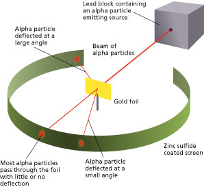
Gold Foil Experiment
Faraday Cage
Oil Drop Experiment
Magnetic Monopole
Why Do Fireflies Light Up
Types of Blood Cells With Their Structure, and Functions
The Main Parts of a Plant With Their Functions
Parts of a Flower With Their Structure and Functions
Parts of a Leaf With Their Structure and Functions
Why Does Ice Float on Water
Why Does Oil Float on Water
How Do Clouds Form
What Causes Lightning
How are Diamonds Made
Types of Meteorites
Types of Volcanoes
Types of Rocks

de Broglie Wavelength

The de Broglie wavelength is a fundamental concept in quantum mechanics that profoundly explains particle behavior at the quantum level. According to de Broglie hypothesis, particles like electrons, atoms, and molecules exhibit wave-like and particle-like properties.

This concept was introduced by French physicist Louis de Broglie in his doctoral thesis in 1924, revolutionizing our understanding of the nature of matter.

de Broglie Equation

A fundamental equation core to de Broglie hypothesis establishes the relationship between a particle’s wavelength and momentum . This equation is the cornerstone of quantum mechanics and sheds light on the wave-particle duality of matter. It revolutionizes our understanding of the behavior of particles at the quantum level. Here are some of the critical components of the de Broglie wavelength equation:

1. Planck’s Constant (h)

Central to this equation is Planck’s constant , denoted as “h.” Planck’s constant is a fundamental constant of nature, representing the smallest discrete unit of energy in quantum physics. Its value is approximately 6.626 x 10 -34 Jˑs. Planck’s constant relates the momentum of a particle to its corresponding wavelength, bridging the gap between classical and quantum physics.

2. Particle Momentum (p)

The second critical component of the equation is the particle’s momentum, denoted as “p”. Momentum is a fundamental property of particles in classical physics, defined as the product of an object’s mass (m) and its velocity (v). In quantum mechanics, however, momentum takes on a slightly different form. It is the product of the particle’s mass and its velocity, adjusted by the de Broglie wavelength.

The mathematical formulation of de Broglie wavelength is

We can replace the momentum by p = mv to obtain

The SI unit of wavelength is meter or m. Another commonly used unit is nanometer or nm.

This equation tells us that the wavelength of a particle is inversely proportional to its mass and velocity. In other words, as the mass of a particle increases or its velocity decreases, its de Broglie wavelength becomes shorter, and it behaves more like a classical particle. Conversely, as the mass decreases or velocity increases, the wavelength becomes longer, and the particle exhibits wave-like behavior. To grasp the significance of this equation, let us consider the example of an electron .

de Broglie Wavelength of Electron

Electrons are incredibly tiny and possess a minimal mass. As a result, when they are accelerated, such as when they move around the nucleus of an atom , their velocities can become significant fractions of the speed of light, typically ~1%.

Consider an electron moving at 2 x 10 6 m/s. The rest mass of an electron is 9.1 x 10 -31 kg. Therefore,

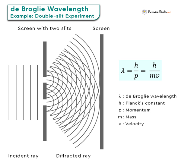
These short wavelengths are in the range of the sizes of atoms and molecules, which explains why electrons can exhibit wave-like interference patterns when interacting with matter, a phenomenon famously observed in the double-slit experiment.

state the de broglie hypothesis and the de broglie equation

Thermal de Broglie Wavelength

The thermal de Broglie wavelength is a concept that emerges when considering particles in a thermally agitated environment, typically at finite temperatures. In classical physics, particles in a gas undergo collision like billiard balls. However, particles exhibit wave-like behavior at the quantum level, including wave interference phenomenon. The thermal de Broglie wavelength considers the kinetic energy associated with particles due to their thermal motion.

At finite temperatures, particles within a system possess a range of energies described by the Maxwell-Boltzmann distribution. Some particles have relatively high energies, while others have low energies. The thermal de Broglie wavelength accounts for this distribution of kinetic energies. It helps to understand the statistical behavior of particles within a thermal ensemble.

Mathematical Expression

The thermal de Broglie wavelength (λ th ) is determined by incorporating both the mass (m) of the particle and its thermal kinetic energy (kT) into the de Broglie wavelength equation:

Here, k is the Boltzmann constant, and T is the temperature in Kelvin.

de Broglie Wave Equation – Chem.libretexts.org
de Broglie Wavelength – Spark.iop.org
de Broglie Matter Waves – Openstax.org
Wave Nature of Electron – Hyperphysics.phy-astr.gsu.edu

Article was last reviewed on Friday, October 6, 2023

Join our Newsletter

Fill your E-mail Address

Related Worksheets

Photons and Matter Waves

De Broglie’s Matter Waves

Samuel J. Ling; Jeff Sanny; and William Moebs

Learning Objectives

By the end of this section, you will be able to:

Describe de Broglie’s hypothesis of matter waves
Explain how the de Broglie’s hypothesis gives the rationale for the quantization of angular momentum in Bohr’s quantum theory of the hydrogen atom
Describe the Davisson–Germer experiment
Interpret de Broglie’s idea of matter waves and how they account for electron diffraction phenomena

$\lambda .$

and the rest mass energy is

${E}_{0}={m}_{0}{c}^{2}=\left(0.65\text{kg}\right){\left(2.998\phantom{\rule{0.2em}{0ex}}×\phantom{\rule{0.2em}{0ex}}{10}^{8}\text{m/s}\right)}^{2}=5.84\phantom{\rule{0.2em}{0ex}}×\phantom{\rule{0.2em}{0ex}}{10}^{16}\text{J.}$

Significance We see from these estimates that De Broglie’s wavelengths of macroscopic objects such as a ball are immeasurably small. Therefore, even if they exist, they are not detectable and do not affect the motion of macroscopic objects.

Check Your Understanding What is de Broglie’s wavelength of a nonrelativistic proton with a kinetic energy of 1.0 eV?

$\lambda \phantom{\rule{0.1em}{0ex}}\text{/}\phantom{\rule{0.1em}{0ex}}2$

This equation is the first of Bohr’s quantization conditions, given by (Figure) . Providing a physical explanation for Bohr’s quantization condition is a convincing theoretical argument for the existence of matter waves.

The Electron Wave in the Ground State of Hydrogen Find the de Broglie wavelength of an electron in the ground state of hydrogen.

Significance We obtain the same result when we use (Figure) directly.

Check Your Understanding Find the de Broglie wavelength of an electron in the third excited state of hydrogen.

$\lambda =2\pi n{a}_{0}=2\text{(}3.324\phantom{\rule{0.2em}{0ex}}\text{Å}\text{)}=6.648\phantom{\rule{0.2em}{0ex}}\text{Å}$

$\text{Δ}V,$

Diffraction lines measured with low-energy electrons, such as those used in the Davisson–Germer experiment, are quite broad (see (Figure) ) because the incident electrons are scattered only from the surface. The resolution of diffraction images greatly improves when a higher-energy electron beam passes through a thin metal foil. This occurs because the diffraction image is created by scattering off many crystalline planes inside the volume, and the maxima produced in scattering at Bragg angles are sharp (see (Figure) ).

Neutron Scattering Suppose that a neutron beam is used in a diffraction experiment on a typical crystalline solid. Estimate the kinetic energy of a neutron (in eV) in the neutron beam and compare it with kinetic energy of an ideal gas in equilibrium at room temperature.

${E}_{T}$

Kinetic energy of ideal gas in equilibrium at 300 K is:

${K}_{T}=\frac{3}{2}{k}_{B}T=\frac{3}{2}\left(8.62\phantom{\rule{0.2em}{0ex}}×\phantom{\rule{0.2em}{0ex}}{10}^{-5}\text{eV}\phantom{\rule{0.1em}{0ex}}\text{/}\phantom{\rule{0.1em}{0ex}}\text{K}\right)\left(300\text{K}\right)=38.8\phantom{\rule{0.2em}{0ex}}\text{MeV}.$

We see that these energies are of the same order of magnitude.

Significance Neutrons with energies in this range, which is typical for an ideal gas at room temperature, are called “thermal neutrons.”

Wavelength of a Relativistic Proton In a supercollider at CERN, protons can be accelerated to velocities of 0.75 c . What are their de Broglie wavelengths at this speed? What are their kinetic energies?

${E}_{0}={m}_{0}{c}^{2}=\left(1.672\phantom{\rule{0.2em}{0ex}}×\phantom{\rule{0.2em}{0ex}}{10}^{-27}\text{kg}\right){\left(2.998\phantom{\rule{0.2em}{0ex}}×\phantom{\rule{0.2em}{0ex}}{10}^{8}\text{m/s}\right)}^{2}=938\phantom{\rule{0.2em}{0ex}}\text{MeV}.$

Check Your Understanding Find the de Broglie wavelength and kinetic energy of a free electron that travels at a speed of 0.75 c .

$\lambda =2.14\phantom{\rule{0.2em}{0ex}}\text{pm;}$

De Broglie’s hypothesis of matter waves postulates that any particle of matter that has linear momentum is also a wave. The wavelength of a matter wave associated with a particle is inversely proportional to the magnitude of the particle’s linear momentum. The speed of the matter wave is the speed of the particle.
De Broglie’s concept of the electron matter wave provides a rationale for the quantization of the electron’s angular momentum in Bohr’s model of the hydrogen atom.
In the Davisson–Germer experiment, electrons are scattered off a crystalline nickel surface. Diffraction patterns of electron matter waves are observed. They are the evidence for the existence of matter waves. Matter waves are observed in diffraction experiments with various particles.

Conceptual Questions

Which type of radiation is most suitable for the observation of diffraction patterns on crystalline solids; radio waves, visible light, or X-rays? Explain.

X-rays, best resolving power

$\text{γ}\text{-rays}$

If an electron and a proton are traveling at the same speed, which one has the shorter de Broglie wavelength?

If a particle is accelerating, how does this affect its de Broglie wavelength?

Why is the wave-like nature of matter not observed every day for macroscopic objects?

negligibly small de Broglie’s wavelengths

What is the wavelength of a neutron at rest? Explain.

Why does the setup of Davisson–Germer experiment need to be enclosed in a vacuum chamber? Discuss what result you expect when the chamber is not evacuated.

to avoid collisions with air molecules

At what velocity will an electron have a wavelength of 1.00 m?

$5.0\phantom{\rule{0.2em}{0ex}}×\phantom{\rule{0.2em}{0ex}}{10}^{6}\text{m/s}$

What is the de Broglie wavelength of an electron that is accelerated from rest through a potential difference of 20 keV?

What is the de Broglie wavelength of a proton whose kinetic energy is 2.0 MeV? 10.0 MeV?

20 fm; 9 fm

What is the de Broglie wavelength of a 10-kg football player running at a speed of 8.0 m/s?

(a) What is the energy of an electron whose de Broglie wavelength is that of a photon of yellow light with wavelength 590 nm? (b) What is the de Broglie wavelength of an electron whose energy is that of the photon of yellow light?

a. 2.103 eV; b. 0.846 nm

The de Broglie wavelength of a neutron is 0.01 nm. What is the speed and energy of this neutron?

What is the wavelength of an electron that is moving at a 3% of the speed of light?

At what velocity does a proton have a 6.0-fm wavelength (about the size of a nucleus)? Give your answer in units of c .

What is the velocity of a 0.400-kg billiard ball if its wavelength is 7.50 fm?

$2.21\phantom{\rule{0.2em}{0ex}}×\phantom{\rule{0.2em}{0ex}}{10}^{\text{−}19}\text{m/s}$

Share This Book

6.5 De Broglie’s Matter Waves

Learning objectives.

By the end of this section, you will be able to:

Describe de Broglie’s hypothesis of matter waves
Explain how the de Broglie’s hypothesis gives the rationale for the quantization of angular momentum in Bohr’s quantum theory of the hydrogen atom
Describe the Davisson–Germer experiment
Interpret de Broglie’s idea of matter waves and how they account for electron diffraction phenomena

According to de Broglie’s hypothesis, massless photons as well as massive particles must satisfy one common set of relations that connect the energy E with the frequency f , and the linear momentum p with the wavelength λ . λ . We have discussed these relations for photons in the context of Compton’s effect. We are recalling them now in a more general context. Any particle that has energy and momentum is a de Broglie wave of frequency f and wavelength λ : λ :

Here, E and p are, respectively, the relativistic energy and the momentum of a particle. De Broglie’s relations are usually expressed in terms of the wave vector k → , k → , k = 2 π / λ , k = 2 π / λ , and the wave frequency ω = 2 π f , ω = 2 π f , as we usually do for waves:

Wave theory tells us that a wave carries its energy with the group velocity . For matter waves, this group velocity is the velocity u of the particle. Identifying the energy E and momentum p of a particle with its relativistic energy m c 2 m c 2 and its relativistic momentum mu , respectively, it follows from de Broglie relations that matter waves satisfy the following relation:

where β = u / c . β = u / c . When a particle is massless we have u = c u = c and Equation 6.57 becomes λ f = c . λ f = c .

Example 6.11

How long are de broglie matter waves.

Depending on the problem at hand, in this equation we can use the following values for hc : h c = ( 6.626 × 10 −34 J · s ) ( 2.998 × 10 8 m/s ) = 1.986 × 10 −25 J · m = 1.241 eV · μ m h c = ( 6.626 × 10 −34 J · s ) ( 2.998 × 10 8 m/s ) = 1.986 × 10 −25 J · m = 1.241 eV · μ m

For the basketball, the kinetic energy is K = m u 2 / 2 = ( 0.65 kg ) ( 10 m/s ) 2 / 2 = 32.5 J K = m u 2 / 2 = ( 0.65 kg ) ( 10 m/s ) 2 / 2 = 32.5 J and the rest mass energy is E 0 = m c 2 = ( 0.65 kg ) ( 2.998 × 10 8 m/s ) 2 = 5.84 × 10 16 J. E 0 = m c 2 = ( 0.65 kg ) ( 2.998 × 10 8 m/s ) 2 = 5.84 × 10 16 J. We see that K / ( K + E 0 ) ≪ 1 K / ( K + E 0 ) ≪ 1 and use p = m u = ( 0.65 kg ) ( 10 m/s ) = 6.5 J · s/m : p = m u = ( 0.65 kg ) ( 10 m/s ) = 6.5 J · s/m : λ = h p = 6.626 × 10 −34 J · s 6.5 J · s/m = 1.02 × 10 −34 m . λ = h p = 6.626 × 10 −34 J · s 6.5 J · s/m = 1.02 × 10 −34 m .
For the nonrelativistic electron, E 0 = m c 2 = ( 9.109 × 10 −31 kg ) ( 2.998 × 10 8 m/s ) 2 = 511 keV E 0 = m c 2 = ( 9.109 × 10 −31 kg ) ( 2.998 × 10 8 m/s ) 2 = 511 keV and when K = 1.0 eV , K = 1.0 eV , we have K / ( K + E 0 ) = ( 1 / 512 ) × 10 −3 ≪ 1 , K / ( K + E 0 ) = ( 1 / 512 ) × 10 −3 ≪ 1 , so we can use the nonrelativistic formula. However, it is simpler here to use Equation 6.58 : λ = h p = h c K ( K + 2 E 0 ) = 1.241 eV · μ m ( 1.0 eV ) [ 1.0 eV+ 2 ( 511 keV ) ] = 1.23 nm . λ = h p = h c K ( K + 2 E 0 ) = 1.241 eV · μ m ( 1.0 eV ) [ 1.0 eV+ 2 ( 511 keV ) ] = 1.23 nm . If we use nonrelativistic momentum, we obtain the same result because 1 eV is much smaller than the rest mass of the electron.
For a fast electron with K = 108 keV, K = 108 keV, relativistic effects cannot be neglected because its total energy is E = K + E 0 = 108 keV + 511 keV = 619 keV E = K + E 0 = 108 keV + 511 keV = 619 keV and K / E = 108 / 619 K / E = 108 / 619 is not negligible: λ = h p = h c K ( K + 2 E 0 ) = 1.241 eV · μm 108 keV [ 108 keV + 2 ( 511 keV ) ] = 3.55 pm . λ = h p = h c K ( K + 2 E 0 ) = 1.241 eV · μm 108 keV [ 108 keV + 2 ( 511 keV ) ] = 3.55 pm .

Significance

Check your understanding 6.11.

What is de Broglie’s wavelength of a nonrelativistic proton with a kinetic energy of 1.0 eV?

Using the concept of the electron matter wave, de Broglie provided a rationale for the quantization of the electron’s angular momentum in the hydrogen atom, which was postulated in Bohr’s quantum theory. The physical explanation for the first Bohr quantization condition comes naturally when we assume that an electron in a hydrogen atom behaves not like a particle but like a wave. To see it clearly, imagine a stretched guitar string that is clamped at both ends and vibrates in one of its normal modes. If the length of the string is l ( Figure 6.18 ), the wavelengths of these vibrations cannot be arbitrary but must be such that an integer k number of half-wavelengths λ / 2 λ / 2 fit exactly on the distance l between the ends. This is the condition l = k λ / 2 l = k λ / 2 for a standing wave on a string. Now suppose that instead of having the string clamped at the walls, we bend its length into a circle and fasten its ends to each other. This produces a circular string that vibrates in normal modes, satisfying the same standing-wave condition, but the number of half-wavelengths must now be an even number k , k = 2 n , k , k = 2 n , and the length l is now connected to the radius r n r n of the circle. This means that the radii are not arbitrary but must satisfy the following standing-wave condition:

If an electron in the n th Bohr orbit moves as a wave, by Equation 6.59 its wavelength must be equal to λ = 2 π r n / n . λ = 2 π r n / n . Assuming that Equation 6.58 is valid, the electron wave of this wavelength corresponds to the electron’s linear momentum, p = h / λ = n h / ( 2 π r n ) = n ℏ / r n . p = h / λ = n h / ( 2 π r n ) = n ℏ / r n . In a circular orbit, therefore, the electron’s angular momentum must be

This equation is the first of Bohr’s quantization conditions, given by Equation 6.36 . Providing a physical explanation for Bohr’s quantization condition is a convincing theoretical argument for the existence of matter waves.

Example 6.12

The electron wave in the ground state of hydrogen, check your understanding 6.12.

Find the de Broglie wavelength of an electron in the third excited state of hydrogen.

In the particular experiment that provided the very first evidence of electron waves (known today as the Davisson–Germer experiment ), they studied a surface of nickel. Their nickel sample was specially prepared in a high-temperature oven to change its usual polycrystalline structure to a form in which large single-crystal domains occupy the volume. Figure 6.19 shows the experimental setup. Thermal electrons are released from a heated element (usually made of tungsten) in the electron gun and accelerated through a potential difference Δ V , Δ V , becoming a well-collimated beam of electrons produced by an electron gun. The kinetic energy K of the electrons is adjusted by selecting a value of the potential difference in the electron gun. This produces a beam of electrons with a set value of linear momentum, in accordance with the conservation of energy:

The electron beam is incident on the nickel sample in the direction normal to its surface. At the surface, it scatters in various directions. The intensity of the beam scattered in a selected direction φ φ is measured by a highly sensitive detector. The detector’s angular position with respect to the direction of the incident beam can be varied from φ = 0 ° φ = 0 ° to φ = 90 ° . φ = 90 ° . The entire setup is enclosed in a vacuum chamber to prevent electron collisions with air molecules, as such thermal collisions would change the electrons’ kinetic energy and are not desirable.

When the nickel target has a polycrystalline form with many randomly oriented microscopic crystals, the incident electrons scatter off its surface in various random directions. As a result, the intensity of the scattered electron beam is much the same in any direction, resembling a diffuse reflection of light from a porous surface. However, when the nickel target has a regular crystalline structure, the intensity of the scattered electron beam shows a clear maximum at a specific angle and the results show a clear diffraction pattern (see Figure 6.20 ). Similar diffraction patterns formed by X-rays scattered by various crystalline solids were studied in 1912 by father-and-son physicists William H. Bragg and William L. Bragg . The Bragg law in X-ray crystallography provides a connection between the wavelength λ λ of the radiation incident on a crystalline lattice, the lattice spacing, and the position of the interference maximum in the diffracted radiation (see Diffraction ).

The lattice spacing of the Davisson–Germer target, determined with X-ray crystallography, was measured to be a = 2.15 Å . a = 2.15 Å . Unlike X-ray crystallography in which X-rays penetrate the sample, in the original Davisson–Germer experiment, only the surface atoms interact with the incident electron beam. For the surface diffraction, the maximum intensity of the reflected electron beam is observed for scattering angles that satisfy the condition n λ = a sin φ n λ = a sin φ (see Figure 6.21 ). The first-order maximum (for n = 1 n = 1 ) is measured at a scattering angle of φ ≈ 50 ° φ ≈ 50 ° at Δ V ≈ 54 V , Δ V ≈ 54 V , which gives the wavelength of the incident radiation as λ = ( 2.15 Å ) sin 50 ° = 1.64 Å . λ = ( 2.15 Å ) sin 50 ° = 1.64 Å . On the other hand, a 54-V potential accelerates the incident electrons to kinetic energies of K = 54 eV . K = 54 eV . Their momentum, calculated from Equation 6.61 , is p = 2.478 × 10 −5 eV · s / m . p = 2.478 × 10 −5 eV · s / m . When we substitute this result in Equation 6.58 , the de Broglie wavelength is obtained as

The same result is obtained when we use K = 54 eV K = 54 eV in Equation 6.61 . The proximity of this theoretical result to the Davisson–Germer experimental value of λ = 1.64 Å λ = 1.64 Å is a convincing argument for the existence of de Broglie matter waves.

Diffraction lines measured with low-energy electrons, such as those used in the Davisson–Germer experiment, are quite broad (see Figure 6.20 ) because the incident electrons are scattered only from the surface. The resolution of diffraction images greatly improves when a higher-energy electron beam passes through a thin metal foil. This occurs because the diffraction image is created by scattering off many crystalline planes inside the volume, and the maxima produced in scattering at Bragg angles are sharp (see Figure 6.22 ).

Since the work of Davisson and Germer, de Broglie’s hypothesis has been extensively tested with various experimental techniques, and the existence of de Broglie waves has been confirmed for numerous elementary particles. Neutrons have been used in scattering experiments to determine crystalline structures of solids from interference patterns formed by neutron matter waves. The neutron has zero charge and its mass is comparable with the mass of a positively charged proton. Both neutrons and protons can be seen as matter waves. Therefore, the property of being a matter wave is not specific to electrically charged particles but is true of all particles in motion. Matter waves of molecules as large as carbon C 60 C 60 have been measured. All physical objects, small or large, have an associated matter wave as long as they remain in motion. The universal character of de Broglie matter waves is firmly established.

Example 6.13

Neutron scattering.

We see that p 2 c 2 ≪ E 0 2 p 2 c 2 ≪ E 0 2 so K ≪ E 0 K ≪ E 0 and we can use the nonrelativistic kinetic energy:

Kinetic energy of ideal gas in equilibrium at 300 K is:

We see that these energies are of the same order of magnitude.

Example 6.14

Wavelength of a relativistic proton, check your understanding 6.13.

Find the de Broglie wavelength and kinetic energy of a free electron that travels at a speed of 0.75 c .

As an Amazon Associate we earn from qualifying purchases.

This book may not be used in the training of large language models or otherwise be ingested into large language models or generative AI offerings without OpenStax's permission.

Want to cite, share, or modify this book? This book uses the Creative Commons Attribution License and you must attribute OpenStax.

Access for free at https://openstax.org/books/university-physics-volume-3/pages/1-introduction

Authors: Samuel J. Ling, Jeff Sanny, William Moebs
Publisher/website: OpenStax
Book title: University Physics Volume 3
Publication date: Sep 29, 2016
Location: Houston, Texas
Book URL: https://openstax.org/books/university-physics-volume-3/pages/1-introduction
Section URL: https://openstax.org/books/university-physics-volume-3/pages/6-5-de-broglies-matter-waves

© Jan 19, 2024 OpenStax. Textbook content produced by OpenStax is licensed under a Creative Commons Attribution License . The OpenStax name, OpenStax logo, OpenStax book covers, OpenStax CNX name, and OpenStax CNX logo are not subject to the Creative Commons license and may not be reproduced without the prior and express written consent of Rice University.

de Broglie Equation Definition

Chemistry Glossary Definition of de Broglie Equation

Chemical Laws
Periodic Table
Projects & Experiments
Scientific Method
Biochemistry
Physical Chemistry
Medical Chemistry
Chemistry In Everyday Life
Famous Chemists
Activities for Kids
Abbreviations & Acronyms
Weather & Climate
Ph.D., Biomedical Sciences, University of Tennessee at Knoxville
B.A., Physics and Mathematics, Hastings College

In 1924, Louis de Broglie presented his research thesis, in which he proposed electrons have properties of both waves and particles, like light. He rearranged the terms of the Plank-Einstein relation to apply to all types of matter.

The de Broglie equation is an equation used to describe the wave properties of matter , specifically, the wave nature of the electron : λ = h/mv , where λ is wavelength, h is Planck's constant, m is the mass of a particle, moving at a velocity v. de Broglie suggested that particles can exhibit properties of waves.

The de Broglie hypothesis was verified when matter waves were observed in George Paget Thomson's cathode ray diffraction experiment and the Davisson-Germer experiment, which specifically applied to electrons. Since then, the de Broglie equation has been shown to apply to elementary particles, neutral atoms, and molecules.

De Broglie Hypothesis
Wave-Particle Duality - Definition
Wave Particle Duality and How It Works
Chemistry Timeline
What Is a Photon in Physics?
J.J. Thomson Atomic Theory and Biography
What Is the Definition of "Matter" in Physics?
Mathematical Properties of Waves
Topics Typically Covered in Grade 11 Chemistry
De Broglie Wavelength Example Problem
Top 10 Weird but Cool Physics Ideas
Electron Definition: Chemistry Glossary
What the Compton Effect Is and How It Works in Physics
Quantum Physics Overview
Photoelectric Effect: Electrons from Matter and Light
Balanced Equation Definition and Examples

38 DeBroglie, Intro to Quantum Mechanics, Quantum Numbers 1-3 (M7Q5)

Introduction.

Bohr’s model explained the experimental data for the hydrogen atom and was widely accepted, but it also raised many questions. Why did electrons orbit at only fixed distances defined by a single quantum number n = 1, 2, 3, and so on, but never in between? Why did the model work so well describing hydrogen and one-electron ions, but could not correctly predict the emission spectrum for helium or any larger atoms? The goal of this section is to answer these questions by introducing electron orbitals, their different energies, and other properties. This section includes worked examples, sample problems, and a glossary.

Learning Objectives for DeBroglie, Intro to Quantum Mechanics, Quantum Numbers 1-3

Illustrate how the diffraction of electrons reveals the wave properties of matter. | Behavior of the Microscopic World and De Broglie Wavelength | Interference Patterns are a Hallmark of Wavelike Behavior |
Recognize that quantum theory leads to discrete energy levels and associated wavefunctions and explain their probabilistic interpretation. | The Quantum Mechanical Model of an Atom |
Describe the energy levels and wave functions for the hydrogen atom using three quantum numbers. | Principal Quantum Number | Azimuthal Quantum Number | Magnetic Quantum Number | Table of Atomic Orbital Quantum Numbers |

| Key Concepts and Summary | Glossary | End of Section Exercises |

Behavior in the Microscopic World and De Broglie Wavelength

We know how matter behaves in the macroscopic world—objects that are large enough to be seen by the naked eye follow the rules of classical physics. A billiard ball moving on a table will behave like a particle: It will continue in a straight line unless it collides with another ball or the table cushion, or is acted on by some other force (such as friction). The ball has a well-defined position and velocity (or a well-defined momentum, p = mv, defined by mass m and velocity v ) at any given moment. In other words, the ball is moving in a classical trajectory. This is the typical behavior of a classical object.

One of the first people to pay attention to the special behavior of the microscopic world was Louis de Broglie. He asked the question: If electromagnetic radiation can have particle-like character (as we saw in an earlier section ), can electrons and other submicroscopic particles exhibit wavelike character? In his 1925 doctoral dissertation, de Broglie extended the wave–particle duality of light that Einstein used to resolve the photoelectric effect paradox to material particles. He predicted that a particle with mass m and velocity v (that is, with linear momentum p ) should also exhibit the behavior of a wave with a wavelength value λ , given by this expression in which h is the familiar Planck’s constant:

λ = [latex]\frac{h}{mv}[/latex] = [latex]\frac{h}{p}[/latex]

This quantity is called the de Broglie wavelength. Unlike the other values of λ discussed in this chapter, the de Broglie wavelength is a characteristic of particles and other bodies, not electromagnetic radiation (note that this equation involves velocity [ v , with units m/s], not frequency [ ν , with units Hz]. Although these two symbols are similar, they mean very different things). Where Bohr had postulated the electron as being a particle orbiting the nucleus in quantized orbits, de Broglie argued that Bohr’s assumption of quantization can be explained if the electron is considered not as a particle, but rather as a circular standing wave such that only an integer number of wavelengths could fit exactly within the orbit ( Figure 1 ).

This figure includes a circle formed from a dashed line. A sinusoidal wave pattern indicated with a solid red line is wrapped around the circle, centered about the edge of the circle. Line segments extend outward from the circle extending through 2 wave crests along the circle. A double ended arrow is drawn between these segments and is labeled, “wavelength, lambda.” A dashed double headed arrow is drawn from the center to the edge of the circle and is labeled, “radius r.”

Interference Patterns are a Hallmark of Wavelike Behavior

Shortly after de Broglie proposed the wave nature of matter, two scientists at Bell Laboratories, C. J. Davisson and L. H. Germer, demonstrated experimentally that electrons can exhibit wavelike behavior by showing an interference pattern for electrons reflecting off a crystal. The same interference pattern is also observed when electrons travel through a regular atomic pattern in a crystal. The regularly spaced atomic layers served as slits that diffract the electrons, as used in other interference experiments. Since the spacing between the layers serving as slits needs to be similar in size to the wavelength of the tested wave for an interference pattern to form, Davisson and Germer used a crystalline nickel target for their “slits,” since the spacing of the atoms within the lattice was approximately the same as the de Broglie wavelengths of the electrons that they used. Figure 2 shows an interference pattern. The wave–particle duality of matter can be seen in Figure 2 by observing what happens if electron collisions are recorded over a long period of time. Initially, when only a few electrons have been recorded, they show clear particle-like behavior, having arrived in small localized packets that appear to be random. As more and more electrons arrived and were recorded, a clear interference pattern that is the hallmark of wavelike behavior emerged. Thus, it appears that while electrons are small localized particles, their motion does not follow the equations of motion implied by classical mechanics, but instead it is governed by some type of a wave equation that governs a probability distribution even for a single electron’s motion. Thus the wave–particle duality first observed with photons is actually a fundamental behavior intrinsic to all quantum particles.

This figure has two parts. Part a shows a diagram of an electron source emitting waves that pass through two narrow slits in a barrier. A wave interference pattern results on the opposite side of the barrier that result in evenly spaced, relatively wide horizontal grey lines on a black surface. The black surface is placed at a distance beyond the barrier. Part b shows an electron source at the far left. Two gold arrows point toward two narrow horizontal slits in a barrier. Around these arrows are many small golden dots. On the right side of the barrier, the gold dots are more widely dispersed. A black surface a distance beyond the barrier shows evenly, yet widely dispersed gold dots. An arrow is present below this black surface and is labeled, “Time.” A second black surface is shown to the right that has many more golden dots that appear to be organizing into a pattern of evenly spaced horizontal line segments. A third black surface is shown even further to the right in which many more gold dots are shown in a very clearly established, evenly spaced pattern of horizontal line segments.

View the Dr. Quantum – Double Slit Experiment cartoon for an easy-to-understand description of wave–particle duality and the associated experiments.

Chemistry in Real Life: Dorothy Hodgkin

Because the wavelengths of X-rays (10-10,000 picometers [pm]) are comparable to the size of atoms, X-rays can be used to determine the structure of molecules. When a beam of X-rays is passed through molecules packed together in a crystal, the X-rays collide with the electrons and scatter. Constructive and destructive interference of these scattered X-rays creates a specific diffraction pattern. Calculating backward from this pattern, the positions of each of the atoms in the molecule can be determined very precisely. One of the pioneers who helped create this technology was Dorothy Crowfoot Hodgkin.

She was born in Cairo, Egypt, in 1910, where her British parents were studying archeology. Even as a young girl, she was fascinated with minerals and crystals. When she was a student at Oxford University, she began researching how X-ray crystallography could be used to determine the structure of biomolecules. She invented new techniques that allowed her and her students to determine the structures of vitamin B 12 , penicillin, and many other important molecules. Diabetes, a disease that affects 382 million people worldwide, involves the hormone insulin. Hodgkin began studying the structure of insulin in 1934, but it required several decades of advances in the field before she finally reported the structure in 1969. Understanding the structure has led to better understanding of the disease and treatment options.

Calculating the Wavelength of a Particle If an electron travels at a velocity of 1.000 × 10 7 m/s and has a mass of 9.109 × 10 –28 g, what is its wavelength?

Solution We can use de Broglie’s equation to solve this problem, but we first must do a unit conversion of Planck’s constant. You learned earlier that 1 J = 1 kg m 2 /s 2 . Thus, we can write h = 6.626 × 10 –34 J·s as 6.626 × 10 –34 kg m 2 /s.

= [latex]\frac{6.626\;\times\; 10^{-34}\;\text{kg m}^{2}\text{/s}}{(9.190\;\times\; 10^{-31} \;\text{kg})(1.000\;\times\; 10^{7}\;\text{m/s})}[/latex]

This is a small value, but it is significantly larger than the size of an electron in the classical (particle) view. This size is the same order of magnitude as the size of an atom. This means that electron wavelike behavior is going to be noticeable in an atom.

Check Your Learning Calculate the wavelength of a softball with a mass of 100 g traveling at a velocity of 35 m/s, assuming that it can be modeled as a single particle.

1.9 × 10 –34 m

We never think of a thrown softball having a wavelength, since this wavelength is so small it is impossible for our senses or any known instrument to detect. The de Broglie wavelength is only appreciable for matter that has a very small mass and/or a very high velocity.

The Quantum–Mechanical Model of an Atom

Shortly after de Broglie published his ideas that the electron in a hydrogen atom could be better thought of as being a circular standing wave instead of a particle moving in quantized circular orbits, as Bohr had argued, Erwin Schrödinger extended de Broglie’s work by incorporating the de Broglie relation into a wave equation, deriving what is today known as the Schrödinger equation. When Schrödinger applied his equation to hydrogen-like atoms, he was able to reproduce Bohr’s expression for the energy and, thus, the Rydberg formula governing hydrogen spectra. He did so without having to invoke Bohr’s assumptions of stationary states and quantized orbits, angular momenta, and energies. Quantization in Schrödinger’s theory was a natural consequence of the underlying mathematics of the wave equation. Like de Broglie, Schrödinger initially viewed the electron in hydrogen as being a physical wave instead of a particle, but where de Broglie thought of the electron in terms of circular stationary waves, Schrödinger properly thought in terms of three-dimensional stationary waves, or wavefunctions , represented by the Greek letter psi, ψ . A few years later, Max Born proposed an interpretation of the wavefunction, ψ, that is still accepted today: Electrons are still particles, and so the waves represented by ψ are not physical waves. However, when you square them, you obtain the probability density which describes the probability of the quantum particle being present near a certain location in space. Wavefunctions, therefore, can be used to determine the distribution of the electron’s density with respect to the nucleus in an atom, but cannot be used to pinpoint the exact location of the electron at any given time. In other words, they predict the energy levels available for electrons in an atom and the probability of finding an electron at a particular place in an atom. Schrödinger’s work, as well as that of Heisenberg and many other scientists following in their footsteps, is generally referred to as quantum mechanics .

You may also have heard of Schrödinger because of his famous thought experiment. This story explains the concepts of superposition and entanglement as related to a cat in a box with poison .

Understanding Quantum Theory of Electrons in Atoms

As was described previously, electrons in atoms can exist only on discrete energy levels but not between them. It is said that the energy of an electron in an atom is quantized, meaning it can be equal only to certain specific values. The electron can jump from one energy level to another, but it cannot transition smoothly because it cannot exist between the levels.

Principal Quantum Number

The energy levels are labeled with an n value, where n = 1, 2, 3, …∞. Generally speaking, the energy of an electron in an atom is greater for greater values of n . This number, n , is referred to as the principal quantum number. The principal quantum number defines the location of the energy level. It is essentially the same concept as the n in the Bohr atom description. Another name for the principal quantum number is the shell number. The shells of an atom can be thought of as concentric circles radiating out from the nucleus. The electrons that belong to a specific shell are most likely to be found within the corresponding circular area (not traveling along the circular ring like a planet orbiting the sun). The further we proceed from the nucleus, the higher the shell number, and so the higher the energy level ( Figure 4 ). The positively charged protons in the nucleus stabilize the electronic orbitals by electrostatic attraction between the positive charges of the protons and the negative charges of the electrons. So the further away the electron is from the nucleus, the greater the energy it has.

This figure contains a central green sphere labeled “nucleus.” There is a plus sign in the middle of the sphere. This sphere is encircled by 3 concentric, evenly spaced rings. The first and closest to the center is labeled, “n equals 1.” The second ring is labeled, “n equals 2,” and the third ring is labeled, “n equals 3.” An arrow is drawn from the edge of the central sphere to the right extending out of the concentric rings. It is labeled, “increasing energy.”

In a major advance over the Bohr theory of the hydrogen atom, in the quantum mechanical model, one can calculate the quantized energies of any isolated atom. Knowing these energies one can then predict the frequencies and energies of photons that are emitted or absorbed based on the difference of the calculated energy levels using the equation presented in the previous quantum, | Δ E | = | E f − E i | = hν. In the case of the hydrogen atom, the expression simplifies to the previously obtained Bohr result.

ΔE = E final – E initial = -2.179 × 10 -18 [latex](\frac{1}{n^2_\text{f}} - \frac{1}{n^2_\text{i}})[/latex] J

The principal quantum number is one of three quantum numbers used to characterize an orbital. An atomic orbital , which is distinct from an orbit , is a general region in an atom within which an electron is most probable to reside. More precisely, the orbital specifies the probability of finding an electron in the three-dimensional space around the nucleus and is based on solutions of the Schrödinger equation. In addition, the principal quantum number defines the energy of an electron in a hydrogen or hydrogen-like atom or an ion (an atom or an ion with only one electron) and the general region in which discrete energy levels of electrons in multi-electron atoms and ions are located.

Angular Momentum Quantum Number

Another quantum number is l , the angular momentum quantum number (this is sometimes referred to as the azimuthal quantum number). It is an integer that defines the shape of the orbital, and takes on the values, l = 0, 1, 2, …, n – 1. We will learn what these shapes are in the next section . This means that an orbital with n = 1 can have only one value of l , l = 0, whereas n = 2 permits l = 0 and l = 1, and so on. The principal quantum number defines the general size and energy of the orbital. The l value specifies the shape of the orbital. Orbitals with the same value of l form a subshell .

Magnetic Quantum Number

Angular momentum is a vector. Electrons with angular momentum can have this momentum oriented in different directions. In quantum mechanics it is convenient to describe the z component of the angular momentum. The magnetic quantum number , called m l, specifies the z component of the angular momentum for a particular orbital. For example, if l = 0, then the only possible value of m l is zero. When l = 1, m l can be equal to –1, 0, or +1. Generally speaking, m l can be equal to the set of numbers [– l , –( l – 1), …, –1, 0, +1, …, ( l – 1), l ] . The total number of possible orbitals with the same value of l (a subshell) is 2 l + 1. Thus, there is one orbital with l = 0 ( m l = 0 is the only orbital), there are three orbitals with l = 1 ( m l = -1, m l = 0, m l = 1 ), five orbitals with l = 2 ( m l = -2, m l = -1, m l = 0, m l = 1, m l = 2 ), and so on.

Rather than specifying all the values of n and l every time we refer to a subshell or an orbital, chemists use an abbreviated system with lowercase letters to denote the value of l for a particular subshell or orbital. Orbitals with l = 0 are called s orbitals (or the s subshell). The value l = 1 corresponds to the p orbitals. For a given n , p orbitals constitute a p subshell (e.g., 3 p subshell if n = 3). The orbitals with l = 2 are called the d orbitals , followed by the f, g, and h orbitals for l = 3, 4, 5, and there are higher values we will not consider. When naming a subshell, it is common to write the principal quantum number ( n) followed by the subshell letter ( s, p, d, f, etc) . For example, when referring to a subshell with n = 4 and l = 2, we would call this the 4 d subshell. We can also say that there are five different 4 d orbitals since there are five values for m l .

As a review, the principal quantum number defines the general value of the electronic energy, with lower values of n indicating lower (more negative) energies and electrons that are closer to the nucleus. The azimuthal quantum number determines the shape of the orbital and we can use s , p , d , f , etc. to designate which subshell the electron is in. And the magnetic quantum number specifies orientation of the orbital in space. Table 1 below provides the possible combinations of n , l , and m l for the first four shells. You’ll notice that every shell does not contain all shapes of orbitals because of the allowable values for the azimuthal quantum number (e.g., there is not a 1 p orbital—only shells higher than n = 1 contain a p subshell).

Working with Shells and Subshells Indicate the number of subshells, the number of orbitals in each subshell, and the values of l and m l for the orbitals in the n = 4 shell of an atom.

Solution For n = 4, l can have values of 0, 1, 2, and 3. Thus, four subshells are found in the n = 4 shell of an atom. For l = 0, m l can only be 0. Thus, there is only one orbital with n = 4 and l = 0. For l = 1, m l can have values of –1, 0, +1, so we find three orbitals. For l = 2, m l can have values of –2, –1, 0, +1, +2, so we have five orbitals. When l = 3, m l can have values of –3, –2, –1, 0, +1, +2, +3, and we can have seven orbitals. Thus, we find a total of 16 orbitals in the n = 4 shell of an atom.

Check Your Learning How many orbitals are in the n = 5 shell?

25 orbitals

Key Concepts and Summary

Macroscopic objects act as particles. Microscopic objects (such as electrons) have properties of both a particle and a wave. Their exact trajectories cannot be determined. The quantum mechanical model of atoms describes the three-dimensional position of the electron in a probabilistic manner according to a mathematical function called a wavefunction, often denoted as ψ . Atomic wavefunctions are also called orbitals and describe the areas in an atom where electrons are most likely to be found.

An atomic orbital is characterized by three quantum numbers. The principal quantum number, n , can be any positive integer. The relative energy of an orbital and the average distance of an electron from the nucleus are related to n . Orbitals having the same value of n are said to be in the same shell. The azimuthal quantum number, l , can have any integer value from 0 to n – 1. This quantum number describes the shape or type of the orbital. Orbitals with the same principal quantum number and the same l value belong to the same subshell. The magnetic quantum number, m l , with 2 l + 1 values ranging from – l to + l , describes the orientation of the orbital in space.

Chemistry End of Section Exercises

How are the Bohr model and the quantum mechanical model of the hydrogen atom similar? How are they different?
Without using quantum numbers, describe the differences between the shells, subshells, and orbitals of an atom.
How do the quantum numbers of the shells, subshells, and orbitals of an atom differ?
Describe the wavefunction and in what ways Schrödinger built upon de Broglie’s previous work.
[latex]c = \lambda\nu[/latex]
[latex]E = h\nu[/latex]
[latex]\lambda = \frac{h}{m\nu}[/latex]

Answers to Chemistry End of Section Exercises

Both models have a central positively charged nucleus with electrons moving about the nucleus in accordance with the Coulomb electrostatic potential. The Bohr model assumes that the electrons move in circular orbits that have quantized energies, angular momentum, and radii that are specified by a single quantum number, n = 1, 2, 3, …, but this quantization is an ad hoc assumption made by Bohr to incorporate quantization into an essentially classical mechanics description of the atom. Bohr also assumed that electrons orbiting the nucleus normally do not emit or absorb electromagnetic radiation, but do so when the electron switches to a different orbit. In the quantum mechanical model, the electrons do not move in precise orbits. There are inherent limitations in determining simultaneously both the position and energy of a quantum particle like an electron, an outcome of the Heisenberg uncertainty principle, so precise orbits are not possible. Instead, a probabilistic interpretation of the electron’s position at any given instant is used, with a mathematical function ψ called a wavefunction that can be used to determine the electron’s spatial probability distribution. These wavefunctions, or orbitals, are three-dimensional stationary waves that can be specified by three quantum numbers that arise naturally from their underlying mathematics (no ad hoc assumptions required): the principal quantum number, n (the same one used by Bohr), which specifies shells such that orbitals having the same n all have the same energy and approximately the same spatial extent; the angular momentum quantum number l , which is a measure of the orbital’s angular momentum and corresponds to the orbitals’ general shapes, as well as specifying subshells such that orbitals having the same l (and n ) all have the same energy; and the orientation quantum number m , which is a measure of the z component of the angular momentum and corresponds to the orientations of the orbitals. The Bohr model gives the same expression for the energy as the quantum mechanical expression and, hence, both properly account for hydrogen’s discrete spectrum (an example of getting the right answers for the wrong reasons, something that many chemistry students can sympathize with), but gives the wrong expression for the angular momentum (Bohr orbits necessarily all have non-zero angular momentum, but some quantum orbitals [ s orbitals] can have zero angular momentum).
(a) Shells describe the general size of an orbital (or distance from the nucleus), subshells describe the shape of an orbital, and the actual orbitals include additional information about the orientation of the orbital; (b) the quantum numbers for shells are integers starting from n = 1, for subshells they are integers with values of 0 … ( n – 1), for orbitals they are integers with values of – l … + l .
Wavefunctions are mathematical functions describing energy and position of electrons in an atom. Building on deBroglie’s work, Schrodinger described the electrons as three-dimensional stationary waves. This was also further extended by Born to show that the square of wavefunction is the probability of finding a quantum particle (electron) in a certain location.
(a) wavelike behavior because it is describing the relationship between wavelength and frequency of a wave; (b) particle-like behavior because it is describing the energy of a particle (photon) with frequency ν; (c) both because it is describing that a particle with mass m can have a wavelength λ.

Share This Book

Making Sense of Quantum Mechanics pp 129–197 Cite as

The de Broglie–Bohm Theory

Jean Bricmont 2
First Online: 13 January 2016

3353 Accesses

1 Citations

3 Altmetric

The de Broglie-Bohm theory, which is a deterministic theory of matter in motion, is explained in this chapter. We first show what the trajectories look like and, then, how to derive the usual quantum predictions, both for the positions of particles and for other observables, using spin and momentum as examples. This derivation rests on the assumption of quantum equilibrium, which we shall explain and discuss. We also see how nonlocality appears in the de Broglie-Bohm theory and we shall present and answer several objections to that theory.

Quantum Equilibrium
Ordinary Quantum Mechanics
Bohmian Mechanics
momentumMomentum
collapseCollapse

These keywords were added by machine and not by the authors. This process is experimental and the keywords may be updated as the learning algorithm improves.

This is a preview of subscription content, log in via an institution .

Buying options

Available as PDF
Read on any device
Instant download
Own it forever
Available as EPUB and PDF
Compact, lightweight edition
Dispatched in 3 to 5 business days
Free shipping worldwide - see info
Durable hardcover edition

Tax calculation will be finalised at checkout

Purchases are for personal use only

In this chapter, we will discuss only the non-relativistic de Broglie–Bohm theory. The issue of relativity (and of quantum fields) will be addressed in Sect. 5.2.2 . By “relativity”, we mean the special theory of relativity, unless the general one is mentioned.

We saw such claims made in Chap. 1 and we will discuss them again in Chap. 7 .

See, e.g., [8, 9, 474] for elementary introductions and [24, 55, 70, 152, 153, 231, 268, 359, 473] for more advanced ones. There are also pedagogical videos made by students in Munich, available at: https://cast.itunes.uni-muenchen.de/vod/playlists/URqb5J7RBr.html .

In Sects. 5.1.3 , 5.1.4 , and 5.2.1 , we will use the presentation of the de Broglie–Bohm theory in Chap. 7 of David Albert’s book Quantum Mechanics and Experience [8].

We let N be the number of variables associated with the system. So if the system consists of M particles moving in three-dimensional space, we have $N=3M$ .

We will call below the pair $\big (\Psi (t), \mathbf{X}(t)\big )$ the state of the system, to be distinguished from the quantum state $\Psi (t)$ , which is only part of it.

The equations here are (partial) differential equations, similar to those discussed in Appendix 2.A. The reader unfamiliar with such equations can skip them and proceed to the remarks. The consequences of these equations will be discussed and illustrated later.

In this chapter, we set $\hbar =1$ . See Appendix 2.A for more details on Schrödinger’s equation .

Of course, in that case, the Schrödinger equation must be replaced by Pauli’s equation , but we will not discuss that (see, e.g., [152, Sect. 8.4]).

The reader familiar with quantum mechanics will recognize the right-hand side of ( 5.1.1.4 ) as the quantum probability current divided by $|\Psi |^2$ . This formula is derived in Appendix 5.A.

A point that is clearly misunderstood by some, e.g., Gisin [214, p. 46]: “If there are hidden positions, there must therefore also be hidden velocities. But that contradicts Heisenberg’s uncertainty principle which is a key part of the quantum formalism [ $\ldots $ ].”.

See, for example, Gouesbet [237, Chap. 17], for an explicit objection to the de Broglie–Bohm theory on that basis.

Setting aside the problems coming from the self-interaction of the particle with its own field.

However, if the wave function is a plane wave , viz., $\Psi (x)= \exp (ikx)$ , a rather idealized situation, then ( 5.1.1.3 ) yields straight line motion with velocity k / m . We will see in the next two subsections that this violation of Newton’s first law does not contradict conservation of momentum , which also holds in quantum mechanics. Indeed, this conservation law concerns results of measurements and the de Broglie–Bohm theory will predict, in a subtle but natural way, the same results of measurements as ordinary quantum mechanics.

For a picture of that potential, see [70, p. 34].

See [151, 362, 522] for a discussion of weak measurements in the context of the de Broglie–Bohm theory.

This does not contradict Heisenberg’s uncertainty relations , because we need to do many operations and take an average to get this result. Heisenberg’s uncertainty relations apply to the results of strong, i.e., ordinary, measurements.

Those theories will be discussed in Sect. 5.4.1 .

See [386, pp. 272–273].

To be mathematically precise, one should add “measurable” or “Borel” here.

Here we use the fact that a function can be defined by giving the value of its integral on every (Borel) subset, if the measure defined by those integrals is absolutely continuous, and we assume here that the map $\phi ^t({\mathbf{x}})$ is such that this measure has this property.

To be precise, this is rather a consequence of what is called equivariance in [141]. See the second part of that appendix.

See Appendix 2.C.

We will take for granted in this subsection that one can detect the positions of particles, and we will see how the de Broglie–Bohm theory accounts for the usual quantum predictions, given that assumption. However, this detection does of course necessitate the coupling of the particle with a macroscopic device, and that coupling, described in conventional terms in Appendix 2.D, will be explained in the context of the de Broglie–Bohm theory in Sect. 5.1.6 and Appendix 5.E.

It should be stressed that all the “experiments” are only meant to illustrate the theory, not to explain how real experiments are performed.

The time evolution is given by Pauli’s equation rather than Schrödinger’s equation . See [152, Sect. 8.4] or [360] for a detailed discussion. The solution given here is similar to the one in Appendix 2.D, except that here we consider the evolution of the wave function of the particle, while in that appendix we considered the evolution of the wave function of the pointer .

One can check that the presence of a magnetic field does not destroy the symmetry $\Psi ( z)=\Psi ( -z)$ .

In that part of the figure, as well as in Fig. 5.6 , the holes are not put in a natural way (top and bottom), but that is just a convention, chosen for graphical convenience.

To be more precise, “blocking” here has to be understood as a collapse of the quantum state, whose meaning, in the de Broglie–Bohm theory, will be explained in the next subsection.

See [38, 69] for further discussion of the “delayed choice” experiment in the de Broglie–Bohm theory.

See Sect. 2.2 and Appendix 2.D.

Englert, Scully, Sussman, and Walther have suggested that the de Broglie–Bohm trajectories are “surrealistic” rather than realistic [175], because those trajectories can have counterintuitive aspects, like the ones discussed here. Originally, the situation described in [175] was presented as an argument against the existence of de Broglie–Bohm trajectories, but in fact those “surrealistic” trajectories can be perfectly understood, in a natural way, within the de Broglie–Bohm theory. See [28, 130, 143, 176, 265] for further discussion of these trajectories.

In our language, where we speak of electrons rather than photons, it would mean that the particles are detected after the arrow with spin up and spin down in the direction 1 half of the time. (Note by J.B.).

The word “contextual” sometimes has a different meaning, as we saw in Appendix 2.F, namely that the result of a measurement may depend on which other measurement is performed simultaneously with the first one. But since one sees here that the result of the “measurement” depends on the details of the apparatus, one can understand that it may also depend on whether another measurement is performed simultaneously. We will come back to this notion of contextuality in Sects. 5.1.5 and 5.3.4 .

Within the de Broglie–Bohm theory, one can introduce, if one wants, “hidden” spin variables, but their value is a function of the quantum state and the positions of the particles (hence, they are redundant) and the actually measured spin values will be affected by the measuring devices and thus not pre-exist their “measurement”. See [268, Chap. 9] or [70, Chap. 10] and references therein for more details on these spin variables.

This is only approximate (hence the use of the symbol $\approx $ below), because of the spreading of the wave functions under free evolution, which implies that, even if the initial wave function has a bounded support, this will not be true at later times. One says that the time evolution produces “tails” of the wave function, namely regions where it is small but nonzero. However, in practice, the probability of finding the particle in one of the tails of the wave function is exceedingly small.

Or, which amounts to the same, with a phase S that is independent of $(x_1,\ldots , x_N)$ . Ground state wave functions are, in general, real.

In [70, Sect. 6.3], Bohm and Hiley give a general analysis of such an interaction. We will discuss only a concrete example.

For another reply, see Gondran and Hoblos [234, 235] who, following Born [77], consider a non-stationary initial wave function and then obtain a de Broglie–Bohm motion close to the classical one.

However, one can even have measurements of the position operator that do not measure positions. See [147, Sect. 7.5] for an example of this situation.

See [147] for a more detailed discussion.

The last sentence is needed because in ordinary quantum mechanics the exact time when the collapse occurs is not well defined. It is defined by the “observation” but, as we discussed before, that notion itself is imprecise.

See Bell [38] for a discussion, similar to the one given here, of the effective collapse of the quantum state in the de Broglie–Bohm theory, but in the example of the double-slit experiment.

It is sometimes thought that, for such an effective collapse to occur, one needs the measuring device to interact with an environment, such as the air molecules surrounding it, and ultimately the entire universe . But that is not true: any sufficiently macroscopic device suffices, even if the latter were perfectly isolated from the rest of the universe (which is never the case, but that is not relevant since what we say would be true even if perfect isolation were possible).

For more details, see, e.g., [80, 225, 307].

There is also the crucial question, which we put aside for now, of what it could mean for the world to be a wave function (see Sect. 6.1 ).

See [185, Chap. 5] and [389, Chap. 7] for pedagogical discussions of this idea.

Assuming that the eigenvalue that is observed is non-degenerate .

We follow the notation of [141] and do not use boldface letters, even though x , y , X , Y generally belong to a space of more than one dimension. This is because we will use boldface letters below for coordinates of several copies of the same system.

In the situations where the decomposition ( 5.1.7.1 ) does not hold, there is a more general notion, the conditional wave function [141]:

where x are the generic variables of the system and Y is the actual position of the environment. Of course, $\Psi (x,Y)=\psi (x) \Phi (Y)$ when the decomposition ( 5.1.7.1 ) holds.

We have $P(X =x|Y=y)= P(X=x,Y=y)/P(Y=y)$ , and $P(Y=y)= \int P(X=x,Y=y)dx = \int |\Psi (x,y)|^2 dx$ . By ( 5.1.7.1 ), if $y\in {\mathrm{supp}\,}\Phi $ , the latter is equal to $\int | \psi (x)\Phi (y)|^2 dx= |\Phi (y)|^2$ , since $\int | \psi (x)|^2 dx=1$ . So finally, $P(X=x,Y=y)/P(Y=y)=| \psi (x)\Phi (y)|^2/|\Phi (y)|^2=|\psi (x)|^2$ .

Nor necessarily at the same time either, although the treatment of measurements at different times is more subtle, see [141, Sects. 8–10].

See Sects. 3.4.4 and 3.4.5 and Appendix 3.A for a definition of those notions.

This convergence to equilibrium cannot be true in full generality since, for any real wave function $\Psi ({\mathbf{x}}) $ nothing moves, hence all distributions are stationary in that situation and do not converge to anything. There have also been some attempts to prove convergence to equilibrium theoretically [67, 481–484].

See [484, 485, 488] for a discussion of a possible non-equilibrium distribution in the early universe.

Indeed, if we perform, say, a position measurement and, as a result we obtain a wave function with a relatively narrow support $\psi (x)$ , then, of course, a subsequent measurement of momentum will start from that wave function and will have a variance $\text{ Var }(p)$ related by ( 2.C.1.4 ) to the variance $\text{ Var }(x)$ of the original x measurement (see Appendix 2.C for the computation of those variances for Gaussian wave functions). On the other hand, if we consider the example of a particle in a box , discussed in Sect. 5.1.4 and Appendix 5.D, the initial momentum is zero and therefore has a variance equal to zero. But, since what we “measure” is not that initial momentum but the asymptotic position of the particle after removing the walls of the box, and thus setting the particle in motion, the result of that “measurement” will coincide with the ordinary quantum predictions (see Appendix 5.D), and will therefore also satisfy the Heisenberg uncertainty relations.

See [141, Sects. 12–14] for more details.

At least according to Wigner , who told the story as though von Neumann was his “friend”, see [516, Note 1, p. 1009].

Here, the probability refers to the Lebesgue measure on the interval [0, 1[, which amounts to considering all the symbols $a_i$ to be independently distributed and giving equal probability to each possible value of $ a_i= 0, \dots , 9$ .

Of course, this assumes a perfect symmetry between the two parts of Fig. 5.11 .

The Schrödinger equation ( 5.1.1.1 ) is also first order in time, but that does not imply that the paths followed by the wave functions cannot cross each other. Indeed, in order for that crossing to be forbidden, one would need the right-hand side of ( 5.1.1.2 ) to coincide for the two wave functions when they cross, i.e., the wave functions and their second derivatives would have to coincide, and there is no reason why that should happen.

The fact that a non-equilibrium distribution would allow us to send messages instantaneously is in fact quite general [486].

And, because of the relativity of simultaneity , discussed in the next subsection, one could in principle send them into one’s own past, at least when one does not introduce an additional structure, such as a preferred foliation into spacetime. See [319, Chap. 4] and [48] for a discussion of the relationship between nonlocality and the sending of messages.

Readers may wonder what “first” and “later” mean in a relativistic framework. This will be discussed in the next subsection.

See [37, 158, 208], [70, p. 139], and [319, Chap. 4] for a general argument.

This is not the way quantum field theory is usually presented, but it allows us to make a straightforward connection with ordinary quantum mechanics.

See [145, 146, 148, 150]. For reviews and references to the original papers, see [464, 465, 477].

See, for example, [216] for an introduction to a rigorous approach to quantum field theories. One can always put a cutoff on the range of momenta to which the theory applies in order to make it well defined, although that trick does not answer the real question, namely, what happens if one removes the cutoff.

This is, of course, an idealization, but it is good enough to allow us to identify approximate inertial frames of reference.

This is because the speed of light enters into those equations. But then the equations cannot be invariant under Galilean transformations, since those transformations change the speed of any object when one passes from one frame to another.

For a good introduction to the theory of relativity, see [469], and for a careful conceptual discussion, see [326].

Under the Lorentz transformations, the speed of light is constant and the laws of electromagnetism are invariant.

At least, since one cannot check experimentally that this simultaneity is absolute , much faster than the speed of light .

Technically, this is called a foliation of spacetime.

For example, when one derives conservation laws , such as conservation of energy , momentum , and angular momentum , one always assumes that the systems to which those laws apply are isolated, otherwise there would be no way to derive those laws. But if the conservation laws held only for the universe, they would have no practical applications.

In ( 2.A.2.24 ), one sees that the larger the mass, the slower the spreading, since time enters in ( 2.A.2.24 ) only through the factor t / m .

For particles in the box, this corresponds to large index n in the wave functions $\Psi _n$ (see Appendix 5.D).

Here are some remarks that may help to understand the quote. The many-worlds theory will be discussed in Sect. 6.1 . The von Neumann theorem will be discussed in Sect. 7.4 . The Kochen –Specker theorem is a version of the theorem in Sect. 2.5 . The curved trajectories in the absence of forces are illustrated in Fig. 5.1 . The stationary quantum states referred to here are those were the wave function is real, whence the particles do not move, according to ( 5.1.1.3 ). In Appendix 5.D, we give examples of such states, even with high energies.

Since their positions vary with time, they also have velocities but, as we discussed in Sect. 5.1.4 , when one “measures” the “momentum ”, one does not get the actual value of those velocities. So in the de Broglie–Bohm theory, there are no “hidden variables ” for the momenta. We will discuss this important property of the de Broglie–Bohm theory again in Sect. 5.3.3 .

Like the particles in the box whose states are discussed in Appendix 5.D, or certain electrons , whose wave function is also real, for example, those in an atomic “ground state”.

See Appendix 5.A for the definition of the probability current. (Note by J.B.).

See [344] for a detailed discussion of this objection, and see also [89].

This holds for any given time t , which we suppress here in the arguments of $\Psi (x)$ and $\hat{\Psi }(p)$ .

See Appendix 2.C.2.

Of course, both the Hamiltonian and the quantum state depend on the existence and the properties of the particles via the potential term in the Hamiltonian or in the Schrödinger equation .

Writing $\Psi =Re^{iS}$ , we get $\log \Psi = \log R+ iS$ and $|\exp (2 \log \Psi )|=R^2 =|\Psi |^2$ .

The title of the next subsection was inspired by [89].

This follows from the observation that, if one adds any term of the form ${\mathbf{j}}({\mathbf{x}}, t)/|\Psi ({\mathbf{x}}, t)) |^2$ to the right-hand side of ( 5.1.1.4 ), where $\nabla \cdot {\mathbf{j}}=0$ , then the $|\Psi ({\mathbf{x}}, t)|^2$ distribution density remains equivariant, because the left-hand side of ( 5.A.1 ) in Appendix 5.A is not modified by the addition of a current of the form ( 5.A.6 ) with $\nabla \cdot {\mathbf{j}}=0$ .

See [464, 465] for a summary of the different possibilities and for references to the original papers.

Here we introduce a distinction between bosons and fermions which is essential in quantum field theory, but which is not discussed elsewhere in this book. Without entering into a detailed discussion, one can think of bosons, e.g., photons , as mediating interactions between particles, and fermions, e.g., electrons , protons, and neutrons, as constituents of ordinary matter.

In [145, 146, 148, 150], one introduces a stochastic process with creation of pairs of particles at random times and a deterministic evolution in-between. In [99], one introduces a deterministic model with a “Dirac sea”.

One could also introduce only fermionic variables and not bosonic ones. This is actually Bell’s approach in [42].

For a discussion of the situation for relativistic de Broglie–Bohm theories, see [269, 270].

This was in Born’s book Natural Philosophy of Cause and Chance [76], since Bell did not read German and von Neumann’s book [496] was only translated into English in 1955. We will discuss Born and von Neumann’s views in Sects. 7.2 and 7.4 .

This equation was first written by Erwin Madelung , who gave it a “hydrodynamic” interpretation [315, 316].

This property is what is called equivariance in [141].

We assume, as in ( 5.1.3.1 ), that the integrals ( 5.C.1.4 ) are absolutely continuous, so that they define the function $\rho ({\mathbf{x}},t)$ . Equation ( 5.C.1.4 ) is similar to ( 5.1.3.1 ), but here it applies to a probability distribution on $ \mathbb {R}^N$ , with N the number of variables of the system, whereas in ( 5.1.3.1 ) it referred to the empirical density in $ \mathbb {R}^3$ . These concepts are different, even if the formulas look similar. The connection between them is made at the end of this appendix.

We consider here each $x_i \in \mathbb {R}$ , but one could also consider ${\mathbf{x}}_i \in \mathbb {R}^3$ .

This wave function could be the effective wave function of those non-interacting identical systems, defined by ( 5.1.7.5 ).

For more details on this example and on similar ones, see Holland [268, Chap. 4] or Bohm and Hiley [70, Sect. 3.6].

This Appendix is based on [268, Sect. 6.5].

Of course, these are eigenvectors of the Hamiltonian , and the corresponding E are its eigenvalues .

The theory of Fourier series implies that the set $\big (\Psi _n(x)\big )^\infty _{n=1}$ forms a basis of $L^2([0,L],dx)$ , but we will not use this fact.

This may seem artificial as a limit, but if we put back factors of $\hbar $ in our equations, it simply means that we take L large compared to the de Broglie wavelength of the particle.

See Sect. 5.1.4 and [172].

One can also check that, in this limiting situation, the acceleration of the particles vanishes, since the velocity is given by $k_n$ , and the quantum potential defined by ( 5.B.6 ) is constant, whence its contribution to ( 5.1.1.5 ) vanishes.

Author information

Authors and affiliations.

IRMP, UCLouvain, Louvain-la-Neuve, Belgium

Jean Bricmont

You can also search for this author in PubMed Google Scholar

Corresponding author

Correspondence to Jean Bricmont .

5.A The Continuity Equation for the $|\Psi |^2$ Distribution

Let us consider Schrödinger’s equation ( 5.1.1.1 ) with H given by ( 5.1.1.2 ). We will first prove the following continuity equation:

where $\nabla = (\partial / \partial x_1, \ldots , \partial / \partial x_N)$ is the gradient, the dot denotes the scalar product, and ${\mathbf{j}}({\mathbf{x}},t)= (j_k ({\mathbf{x}}, t))_{k=1}^N$ (we index the components here by k instead of j ) is the “probability current” or the “quantum flux” defined by

To prove ( 5.A.1 ), write

take the complex conjugate of ( 5.1.1.1 ), viz.,

and insert this and ( 5.1.1.1 ) into ( 5.A.3 ). The potential term cancels out and we get

It is enough to observe that

to obtain ( 5.A.1 ).

Now, if we consider ( 5.1.1.4 ), we see that the function ${\mathbf{j}}({\mathbf{x}},t)= (j_k ({\mathbf{x}}, t))_{k=1}^N$ [whose arguments are the generic variables ${\mathbf{x}}$ rather than the actual positions of the particles as in ( 5.1.1.4 )] is of the form

and we can write ( 5.A.1 ) as

which is the continuity equation Footnote 97 one would obtain for a “fluid” of density $\rho ({\mathbf{x}},t)=|\Psi ({\mathbf{x}},t)|^2$ , with local velocity ${\mathbf{V}}_{\Psi } ({\mathbf{x}},t)$ . This will be useful when we come to prove the equivariance of the $|\Psi ({\mathbf{x}},t)|^2$ distribution in Appendix 5.C.

5.B A Second Order Dynamics and the Quantum Potential

Here we derive ( 5.1.1.5 ) from ( 5.1.1.1 )–( 5.1.1.3 ). We insert $\Psi ({\mathbf{x}},t)=R({\mathbf{x}},t)e^{iS({\mathbf{x}},t)}$ into Schrödinger’s equation ( 5.1.1.1 ), where ${\mathbf{x}}= (x_1, \dots , x_N)$ . Suppressing here the arguments $({\mathbf{x}}, t)$ , we get

Dividing both sides by $e^{iS}$ and separating the real and imaginary parts give rise to two equations:

Dividing ( 5.B.2 ) by R gives

Multiplying ( 5.B.3 ) by 2 R gives

which, with $R^2=|\Psi |^2$ and using ( 5.A.6 ), is the same as ( 5.A.1 ).

Now, if we consider ( 5.1.1.3 ) and take its time derivative, remembering that S depends on time through $\big (X_1(t),\ldots ,X_N(t)\big )$ and t , we get

If we use ( 5.1.1.3 ) to replace $\dot{X}_j$ by $(1/m_j)(\partial S/\partial x_j)$ in ( 5.B.5 ), and insert ( 5.B.4 ) in the second term of ( 5.B.5 ), evaluating the functions at $\mathbf{X}$ instead of $\mathbf{x}$ , the terms

cancel each other and we get

where the quantum potential Q is given by

This proves ( 5.1.1.5 ).

5.C Proof of the Equivariance of the $|\Psi ({\mathbf{x}},t)|^2$ Distribution

5.1.1 5.c.1 equivariance in $\mathbb {r}^n$.

We will first prove Footnote 98 that, for a system in $\mathbb {R}^N$ and $\forall A \subset \mathbb {R}^N$ ,

provided that, at $t=0$ , $\forall A \subset \mathbb {R}^N$ ,

In ( 5.C.1.1 ), the left-hand side involves ${\mathbf{X}}(t)$ , the solution of ( 5.1.1.4 ), while on the right-hand side, $\Psi ({\mathbf{x}},t)$ is the solution of Schrödinger’s equation ( 5.1.1.1 ).

Consider first a general differential equation

with ${\mathbf{X}}:\mathbb {R}\rightarrow \mathbb {R}^N$ . We assume that ${\mathbf{V}}$ is such that ( 5.C.1.3 ) has solutions for all times. Let $\phi ^t({\mathbf{x}})$ denote the solution at time t of ( 5.C.1.3 ) with initial condition ${\mathbf{X}}(0)= {\mathbf{x}}$ at time 0. Then, given any probability density $\rho ({\mathbf{x}}, 0)$ on the initial conditions ${\mathbf{X}}(0)={\mathbf{x}}$ , define Footnote 99 $\rho ({\mathbf{x}},t)$ , $\forall A \subset \mathbb {R}^N$ , by

where ${\mathbbm {1}}_A$ is the indicator function of the set A .

Then we have

To prove ( 5.C.1.5 ), observe that, by approximating integrals by sums, for any smooth function with compact support, we get from ( 5.C.1.4 ):

Then, differentiating both sides of ( 5.C.1.6 ) with respect to t , and using the fact that ( 5.C.1.3 ) implies $\partial \phi ^t ({\mathbf{x}})/\partial t = {\mathbf{V}}\big (\phi ^t ({\mathbf{x}}), t\big )$ , we have

Using ( 5.C.1.6 ) with $F (\cdot )$ replaced by ${\mathbbm {\nabla }} F (\cdot ) \cdot {\mathbf{V}}(\cdot ,t)$ , the right-hand side of this equals

Integrating by parts, this is

Since ( 5.C.1.7 ) is valid for any F , it implies ( 5.C.1.5 ).

Now, if we consider the differential equation ( 5.C.1.3 ) with ${\mathbf{V}}({\mathbf{X}},t)={\mathbf{V}}_{\Psi } ({\mathbf{X}}, t)$ , with ${\mathbf{V}}_{\Psi } ({\mathbf{X}}, t)$ given by ( 5.1.1.4 ), and $\rho ({\mathbf{x}},t)=|\Psi ({\mathbf{x}},t)|^2$ , we get, using ( 5.C.1.4 ), ( 5.C.1.5 ), and ( 5.A.7 ),

which proves ( 5.C.1.1 ) if we assume that ( 5.C.1.1 ) holds at $t=0$ , which is ( 5.C.1.2 ).

5.1.2 5.C.2 Proof of Equivariance of the Empirical Distributions

To finish the proof of ( 5.1.3.2 ), consider a large number N of copies of non-interacting identical systems, Footnote 100 whose initial wave function Footnote 101 is

The density of the associated probability distribution is

which means that the variables $x_i$ are independent identically distributed random variables with distribution $|\psi (x, 0)|^2$ . This implies, by the law of large numbers (see Appendix 3.A), that the empirical density distribution $\rho (x,0)$ of the N particles will be given, as $N\rightarrow \infty $ , by $\rho (x,0)= |\psi (x, 0)|^2$ .

By ( 5.C.1.1 ), the probability distribution density of $(x_1, \dots , x_N)$ at time $t>0$ will be

and the empirical density distribution $\rho (x,t)$ of the N particles at time t will be given, as $N\rightarrow \infty $ , by $\rho (x,t)= |\psi (x, t)|^2$ . This completes the proof of ( 5.1.3.2 ).

5.D Examples of de Broglie–Bohm Dynamics

5.1.1 5.d.1 the gaussian wave function.

Consider the time evolution of a Gaussian wave function ( 2.A.2.23 ), with initial condition $ \Psi (x, 0)=\pi ^{-1/4}\exp (- x^2/2)$ , which we copy here Footnote 102 :

It is easy to see that, if we write $\Psi (x,t)= R (x,t) \exp \big [iS (x,t)\big ]$ , we have (up to a constant term)

so that ( 5.1.1.3 ) gives rise to the equation of motion

which can be easily integrated by a separation of variables:

This gives the explicit dependence of the position at time t on the initial condition and shows that the particle does not move if it is initially at $X(0)=0$ , but moves asymptotically, when $t\rightarrow \infty $ , according to $X(t)\sim X(0)t/m$ .

Equation ( 2.A.3.3 ) can be checked explicitly here. Indeed, putting $m=1$ as in Appendix 2.A.3, we get from ( 2.A.2.24 )

whose limit as $t \rightarrow \infty $ is $\pi ^{-1/2}\exp (- p^2) =|\widehat{\Psi }(p,0)|^2$ .

It is also easy to verify explicitly the property ( 5.1.3.2 ) of equivariance. From ( 5.D.1.3 ), we get $\phi ^t(x)= x \sqrt{1+(t/m)^2}$ . If we make the change of variable $y= \phi ^t(x)$ in the integral on the right-hand side of ( 5.1.3.1 ), we get, with the initial distribution $\rho (x,0)= | \Psi (x,0)|^2= \pi ^{-1/2}\exp (- x^2)$ ,

Changing the y variable back to x , this coincides with $| \Psi (x,t)|^2$ given by ( 2.A.2.24 ), with the prefactor $1/\sqrt{1+(t/m)^2}$ coming from $dx= dy/\sqrt{1+(t/m)^2}$ .

5.1.2 5.D.2 The Particle in a Box

Consider a particle in a box, Footnote 103 in one dimension, of size L , chosen to be the interval [0, L ]. The particle is free in the box, but constrained to remain in it. Let us look for solutions of the Schrödinger equation ( 5.1.1.1 ), with $N=1$ , of the form $\exp (-iEt) \Psi (x) $ , whose associated probability distribution $|\exp (-iEt) \Psi (x)|^2= | \Psi (x)|^2 $ is independent of time. Footnote 104

We model the presence of the box by setting the potential in ( 5.1.1.2 ) such that $V=0$ inside the box and $V=\infty $ outside the box, which means that $\Psi (x)$ vanishes outside V . So we have to solve

with $\Psi (0) = \Psi (L)=0$ . We have set the mass $m=1$ .

The general solution of ( 5.D.2.1 ) is

and the conditions $\Psi (0)=\Psi (L)=0$ imply $A=-B$ and $E_n=n^2\pi ^2/ L^2$ , for $n\in \mathbbm {Z}$ , $n \ne 0$ . From ( 5.D.2.2 ), we get the eigenvectors

where ${\mathbbm {1}}_{[0, L]} $ is the indicator function of [0, L ], and $k_n = n\pi /L$ . The sine function being odd, we can restrict ourselves to $n=1,2,\ldots , \infty $ , since the solution should be nonzero and is defined up to a multiplicative factor which does not affect the motion of the particle, as can be seen from ( 5.1.1.4 ). Footnote 105 The factor $\sqrt{2/L}$ ensures that $\int _{\mathbbm {R}} |\Psi _n(x)|^2 dx =1$ .

If we take a function $\Psi _n(x)$ as initial condition in ( 5.1.1.1 ), then the time-dependent solution is

Now comes the apparent paradox: the phase $S_n$ of $\Psi _n (x,t)$ is constant in x , so $\partial S_n / \partial x=0$ , and by ( 5.1.1.3 ), the particle is at rest in the box. Let us see how to solve that paradox. As we said, one method to measure the momentum is to remove the walls of the box and to detect the position x of the particle after a certain time t , and give x / t as a “measure” of momentum.

To see what happens when the walls of the box are removed, we have to compute the time evolution of the wave function with initial condition ( 5.D.2.3 ). Since the walls are removed, the time evolution is governed by the free Schrödinger equation ( 5.1.1.1 ). The solution is therefore obtained from ( 2.A.2.21 ) and we need to compute $\widehat{\Psi }(p,0)$ from ( 5.D.2.3 ), leaving out the index n on $\Psi $ . Thus,

Writing $\sin (k_n x) = (e^{ik_n x}-e^{-ik_n x})/2i$ , making the change of variable $x=x'+L/ 2$ , and integrating over $x'\in [-L/ 2,L/ 2]$ , we obtain

This can be written as:

since $e^{-ik_nL}= e^{-in\pi }=(-1)^n$ . From ( 2.A.2.21 ) we get, using the variable $x'=x - L/2$ ,

From Plancherel’s theorem [see also ( 2.A.2.26 )], we know that

Now, for $t\ne 0$ , if we write $\Psi (x',t)=R (x',t) e^{iS(x',t)}$ , there is no reason why we should have $\partial S(x',t)/\partial x'=0$ and an analysis of ( 5.D.2.8 ) shows that we do indeed have $\partial S(x',t)/ \partial x'\ne 0$ for $t\ne 0$ . In fact, we can see this indirectly using ( 2.A.3.2 ) and ( 2.A.3.3 ), which imply

This means that the support of $\Psi (x',t)$ spreads as $t \rightarrow \infty $ (away from $x'=0$ , i.e., away from the center of the box $x=L/ 2$ ), and by equivariance ( 5.1.3.1 ), this means that the particles will move towards either $+\infty $ or $-\infty $ .

To illustrate this, consider what happens in the limit of large n , L (mathematically, $n, L \rightarrow \infty $ ) with $k_n = n\pi / L$ fixed. Footnote 106 It is well known (from the theory of Fourier transforms) that

as $L\rightarrow \infty $ , in the sense of distributions. So in that limit, we may change variables $y=p-k_n$ or $y=p+k_n$ in ( 5.D.2.8 ) and, to a good approximation, replace the integral in ( 5.D.2.8 ) by the value of the factor $\exp (it p^2/2+ipx) $ at $p=\pm k_n$ . We then obtain

which represents two plane waves propagating in opposite directions with absolute velocity $k_n$ , since $\partial (\pm k_n x')/\partial x'= \pm k_n$ .

Of course, one has to be a bit careful with this limit, since we have $L\rightarrow \infty $ and $1/\sqrt{ L}$ in ( 5.D.2.11 ). But the function in square brackets in ( 5.D.2.11 ) is not square integrable over $\mathbbm {R}$ (while we know that $\int _{\mathbbm {R}} |\Psi (x',t) |^2 dx'=1$ for all t ), and moreover, its phase is constant in $x'$ . So what the limit means is that, for large t , $\Psi (x',t)$ is the sum of two square integrable functions, one whose Fourier transform is localized near $p=k_n$ , and the other whose Fourier transform is localized around $p=-k_n$ . And by ( 5.D.2.8 ) and equivariance, we find that the particles that are in the support of one of those two wave functions move with a speed approximately equal to $\pm k_n$ .

The result ( 5.D.2.11 ) is exactly what Einstein asked for, when he thought of the classical limit as being made of a motion going back and forth between the walls of the box, Footnote 107 except that here this only happens once we remove the walls of the box. Footnote 108

5.E The Effective Collapse of the Quantum State and Decoherence

Let us describe the measurement process of Appendix 2.D in more detail (here we follow [70, Sect. 6.1]). When the particle is deflected by the magnetic field , either up or down, its presence is detected by a macroscopic device. One example of such a device would be, for a charged particle, an ion chamber. A cascade of ionization of atoms will eventually produce a pulse that can be observed, at a macroscopic level, by a galvanometer.

Consider two measuring devices, one detecting the particle if it goes up, and one detecting it if it goes down. Let the initial wave function for the two devices be

where $x_1 \ldots x_N$ are the coordinates of the particles making up the first device and $y_1 \ldots y_N$ are those for the second device, while N is of the order of the Avogadro number $(N\sim 10^{23})$ . Let $\Phi ^{\text {{up}}}_\mathrm{f} (x_1,\ldots ,x_N)$ and $ \Phi _\mathrm{f}^{\text {{down}}} (y_1,\ldots ,y_N)$ (f for “final”) denote the wave functions of the detector after the particle has been detected. Note that these wave functions have a support that is disjoint from the support of $\Phi _0^{\text {{up}}}$ , $\Phi _0^{\text {{down}}}$ for each variable $x_i$ , $y_i$ . Indeed, if we think of an ion chamber, then the electrons lost by the ions will move towards an electric plate in $\Phi _\mathrm{f}^{\text {{up}}}$ , while they will remain bound to their atoms in $\Phi _0^{\text {{up}}}$ (and the same holds for $\Phi _0^{\text {{down}}}$ , $\Phi _\mathrm{f}^{\text {{down}}}$ ). But this can occur only if the supports of the wave functions are disjoint, for each electron .

If the initial quantum state of the particle is given by ( 5.1.4.7 ), then the combined initial quantum state of the particle and the ion chamber is

Then, the final quantum state [see ( 5.1.4.8 )] will be:

where we have left out the arguments of the wave functions $\Phi ^{\text {{up}}}_\mathrm{f} \Phi ^{\text {{down}}}_0 $ and $\Phi ^{\text {{up}}}_0 \Phi ^{\text {{down}}}_\mathrm{f}$ . This means that, for the $\Psi (z-t) c_1 |1 \uparrow \rangle $ part of the quantum state, the up detector will be activated and the down part will remain in its original state, and vice versa for the $\Psi (z+t) c_2 |1 \downarrow \rangle $ part.

Now, since the two parts in ( 5.E.2 ) have disjoint supports, the original particle can only be in one of them, and so will be guided only by that part of the quantum state in whose support it happens to lie. However, we cannot generally neglect the part of the wave function in the support of which the particle is not located, because the two parts could subsequently be brought together, in such a way that their supports overlap . This is exactly what causes the interference phenomena, exemplified by the Mach–Zehnder interferometer , as discussed in Sect. 2.2 . In our example, the quantum state of the particle, viz.,

evolves into

where $\Psi (z-t)$ and $\Psi (z+t)$ have disjoint supports (for t not too small). In a quantum state like ( 5.E.3 ), the particle is guided by $\Psi (z-t)$ or $\Psi (z+t)$ , depending on where it is, but we cannot “reduce” the quantum state and keep only that part, because $\Psi (z-t)$ and $\Psi (z+t)$ may later evolve into wave functions with overlapping supports.

But how can one do that with a quantum state like ( 5.E.2 ) involving of the order of $10^{23}$ particles? It is not enough to make $\Psi (z-t)$ and $\Psi (z+t)$ overlap, we need to do that also with $\Phi ^{\text {{up}}}_\mathrm{f}$ $\Phi ^{\text {{down}}}_0$ and $\Phi ^{\text {{up}}}_0$ $\Phi ^{\text {{down}}}_\mathrm{f}$ . But this is impossible in practice. Let us see why.

Remember that these wave functions represent a collection of $N\sim 10^{23}$ particles, all of which have different locations, some moving more or less freely and some being bound to their atoms. Hence, the wave functions must have different supports for each particle. Consider, for simplicity, a wave function that factorizes :

and similarly for $\Phi ^{\text {{up}}}_\mathrm{f}$ , $\Phi ^{\text {{down}}}_0 $ , and $\Phi ^{\text {{down}}}_\mathrm{f}$ . The support of $\Phi _{0 i}$ is disjoint from the support of $\Phi _{\mathrm{f} i}$ for every particle since, in the support of $\Phi _{0 i}$ , the particle is bound to the atom and, in the support of $\Phi _{\mathrm{f} i}$ , it is moving.

For the two wave functions to interfere again, we need the wave functions $\Phi _{0 i}(x_i)$ of all the particles to overlap in the future. Indeed, $\Phi ^{\text {{up}}}_0$ and $\Phi ^{\text {{up}}}_\mathrm{f}$ have disjoint supports if

$\forall (x_1, \ldots , x_N) \in {{\mathbb {R}}}^N$ . Of course, the same equation also holds for $\Phi ^{\text {{down}}}_0(x_1, \ldots , x_N)\Phi ^{\text {{down}}}_\mathrm{f}(x_1, \ldots , x_N)$ . But for ( 5.E.5 ) to be true, it is enough to have $\Phi _{0 i} (x_i) \Phi _{\mathrm{f} i}(x_i)=0$ , $\forall x_i \in {{\mathbb {R}}}$ , for a single value of i . Hence, for interference to occur, we need to get the wave functions of every particle in (say) the ion chamber to overlap again.

It is clear that this is, in practice, impossible. The same is true for the particles constituting the live cat and the dead cat, the pointer pointing up or down, the exploded and unexploded bomb, etc. Now, of course, once the position of the original particle is in the support of one of the two terms in ( 5.E.2 ), we can simply reduce the quantum state to that term, since we can be sure that the other term will never again interfere with it.

But we can know in which of the supports of the two terms the particle happens to be located simply by looking at the (by definition) macroscopic result. Hence, in some sense, we do “collapse ” the quantum state after we look at the result of an experiment. However, this is an entirely practical matter. We can still consider, if we wish, that the true quantum state is and remains forever given by the time evolution of ( 5.E.2 ). Put simply, there is one of the terms that does not guide the motion of the particle, either now or ever again.

5.F Proof of the Factorization Formula

We now prove ( 5.1.7.5 ). Note that ( 5.1.7.4 ) implies that

where $\hat{x}_i = (x_1,\ldots ,x_M)$ with $x_i$ missing and we have put in $\Phi _i(\hat{x}_i, {\mathbf{Y}})$ the arguments that were not indicated in ( 5.1.7.4 ).

To prove ( 5.1.7.5 ), consider $M=2$ . By ( 5.F.1 ), we have

Dividing by $\psi (x_1)\psi (x_2)$ , we get

which means that both sides are functions of ${\mathbf{Y}}$ alone, which we can write $\Phi ({\mathbf{Y}})$ . Thus,

which is ( 5.1.7.5 ) for $M=2$ . The argument easily extends to all M .

Rights and permissions

Reprints and permissions

Copyright information

About this chapter

Cite this chapter.

Bricmont, J. (2016). The de Broglie–Bohm Theory. In: Making Sense of Quantum Mechanics. Springer, Cham. https://doi.org/10.1007/978-3-319-25889-8_5

Download citation

DOI : https://doi.org/10.1007/978-3-319-25889-8_5

Published : 13 January 2016

Publisher Name : Springer, Cham

Print ISBN : 978-3-319-25887-4

Online ISBN : 978-3-319-25889-8

eBook Packages : Physics and Astronomy Physics and Astronomy (R0)

Share this chapter

Anyone you share the following link with will be able to read this content:

Sorry, a shareable link is not currently available for this article.

Provided by the Springer Nature SharedIt content-sharing initiative

Publish with us

Policies and ethics

Find a journal
Track your research

school Campus Bookshelves
menu_book Bookshelves
perm_media Learning Objects
login Login
how_to_reg Request Instructor Account
hub Instructor Commons
Download Page (PDF)
Download Full Book (PDF)
Periodic Table
Physics Constants
Scientific Calculator
Reference & Cite
Tools expand_more
Readability

selected template will load here

This action is not available.

2.5: The de Broglie-Bohr Model for the Hydrogen Atom - Version 4

Last updated
Save as PDF
Page ID 154850

Frank Rioux
College of Saint Benedict/Saint John's University

The 1913 Bohr model of the hydrogen atom was replaced by Schrödingerʹs wave mechanical model in 1926. However, Bohrʹs model is still profitably taught today because of its conceptual and mathematical simplicity, and because it introduced a number of key quantum mechanical ideas such as the quantum number, quantization of observable properties, quantum jump and stationary state.

Bohr calculated the manifold of allowed electron energies by balancing the mechanical forces (centripetal and electron‐nucleus) on an electron executing a circular orbit of radius R about the nucleus, and then arbitarily quantizing its angular momentum. Finally by fiat he declared that the electron was in a non‐radiating stationary state because an orbiting (accelerating) charge radiates energy and will collapse into the oppositely charge nucleus.

In 1924 de Broglie postulated wave‐particle duality for the electron and other massive particles, thereby providing the opportunity to remove some of the arbitariness from Bohrʹs model. For example, an electron possessing wave properties is subject to constructive and destructive interference. As will be shown this leads naturally to quantization of electron momentum and kinetic energy, and consequently a manifold of allowed energy states for the electron relative to the nucleus. The de Broglie‐Bohr model of the hydrogen atom presented here treats the electron as a particle on a ring with wave‐like properties.

\[ \lambda = \frac{h}{m_e v} \nonumber \]

de Broglie's hypothesis that matter has wave-like properties.

\[n \lambda = 2 \pi r \nonumber \]

The consequence of de Broglieʹs hypothesis; an integral number of wavelengths must fit within the circumference of the orbit. This introduces the quantum number which can have values 1,2,3,... The n = 4 electron state is shown below.

Screen Shot 2019-06-05 at 12.57.30 PM.png

\[ m_e v = \frac{n h }{2 \pi r} \nonumber \]

Substitution of the first equation into the second equation reveals that momentum is quantized.

\[ T = \frac{1}{2} m_e v^2 = \frac{n^2 h^2}{8 \pi^2 m_e r^2} \nonumber \]

If momentum is quantized, so is kinetic energy.

\[ E = T + V = \frac{n^2 h^2}{8 \pi^2 m_e r^2} - \frac{e^2}{4 \pi \varepsilon_0 r} \nonumber \]

Which means that total energy is quantized. The second term is the electron‐proton electrostatic potential energy.

The quantum mechanical interpretation of these ʺBohr orbitsʺ is that they are stationary states. In spite of the fact that we use the expression kinetic energy, which implies electron motion, there is no motion. The electron occupies the orbit as a particle‐wave, it is not orbiting the nucleus. If it was orbiting in a classical sense it would radiate energy and quickly collapse into the nucleus. Clearly the stability of matter requires the quantum mechanical version of kinetic energy.

The ground state energy and orbit radius of the electron in the hydrogen atom is found by plotting the energy as a function of the orbital radius. The ground state is the minimum in the total energy curve. Naturally calculus can be used to obtain the same information by minimizing the energy with respect to the orbit radius. However, the graphical method has the virtue of illuminating the issue of atomic stability.

Fundamental constants: electron charge, electron mass, Planck's constant, vacuum permitivity.

\[ \begin{matrix} e = 1.6021777 (10)^{-19} \text{coul} & m_e = 9.10939 (10)^{-31} \text{kg} \\ h = 6.62608 (10)^{-34} \text{joule sec} & \varepsilon_0 = 8.85419 (10)^{-12} \frac{ \text{coul}^2}{ \text{joule m}} \end{matrix} \nonumber \]

Quantum number and conversion fact between meters and picometers and joules and attojoules.

\[ \begin{matrix} n = 1 & pm = 10^{-12} m & \text{ajoule} = 10^{-18} \text{joule} \end{matrix} \nonumber \]

\[ \begin{matrix} r = 20 pm,~20.5 pm,~ 500 pm & T(r) = \frac{n^2 h^2}{8 \pi^2 m_e r^2} & V(r) = - \frac{e^2}{4 \pi \varepsilon_0 r} & E(r) = T(r) + V(r) \end{matrix} \nonumber \]

Screen Shot 2019-06-05 at 1.04.24 PM.png

This figure shows that atomic stability involves a balance between potential and kinetic energy. The electron is drawn toward the nucleus by the attractive potential energy interaction (~ ‐1/R), but is prevented from collapsing into the nucleus by the extremely large kinetic energy (~1/R2) associated with small orbits.

As shown below, the graphical approach can also be used to find the electronic excited states.

\[ \begin{matrix} n = 2 & T(r) = \frac{n^2 h^2}{8 \pi^2 m_e r^2} & V(r) = - \frac{e^2}{4 \pi \varepsilon_0 r} & E(r) = T(r) + V(r) \end{matrix} \nonumber \]

Screen Shot 2019-06-05 at 1.06.43 PM.png

As mentioned earlier the manifold of allowed electron energies can also be obtained by minimizing the energy with respect to the orbit radius. This procedure yields,

\[ \begin{matrix} E_n = - \frac{m_e e^4}{2 \left(4 \pi \varepsilon_0 \right)^2 \hbar^2 } \frac{1}{n^2} & \text{and} & r_n = \frac{4 \pi \varepsilon_0 \hbar^2}{m_e e^2} n^2 \end{matrix} \nonumber \]

What is De Broglie Hypothesis?

De broglie's hypothesis says that matter consists of both the particle nature as well as wave nature. de broglie wavelength λ is given as λ = h p , where p represents the particle momentum and can be written as: λ = h m v where, h is the planck's constant, m is the mass of the particle, and v is the velocity of the particle. from the above relation, it can be said that the wavelength of the matter is inversely proportional to the magnitude of the particle's linear momentum. this relation is applicable to both microscopic and macroscopic particles the de broglie equation is one of the equations that is commonly used to define the wave properties of matter. electromagnetic radiation exhibits the dual nature of a particle (having a momentum) and wave (expressed in frequency, and wavelength)..

IMAGES

De Broglie Hypothesis
PPT
Which Is The De Broglie Equation?
de Broglie equation
de Broglie Equation
How to Calculate the de Broglie Wavelength of an Electron

VIDEO

De Broglie equation
De-Broglie Hypothesis Experimental Verification
State de-Broglie hypothesis
DE BROGLIE HYPOTHESIS || DUAL NATURE OF MATTER|| CLASS 12 CBSE, JEE, NEET
Lesson 1A 3 de Broglie Hypothesis 2
De Broglie Hypothesis || Wave Nature of Matter || de Broglie Wavelength Physics -2023 ||apniPhysics

COMMENTS

6.6: De Broglie's Matter Waves
In 1924, Louis de Broglie proposed a new speculative hypothesis that electrons and other particles of matter can behave like waves. Today, this idea is known as de Broglie's hypothesis of matter waves. In 1926, De Broglie's hypothesis, together with Bohr's early quantum theory, led to the development of a new theory of wave quantum ...
De Broglie Equation
The wave which is associated with the particles that are moving are known as the matter-wave, and also as the De Broglie wave. The wavelength is known as the de Broglie wavelength. For an electron, de Broglie wavelength equation is: λ = \ [\frac {h} {mv}\] Here, λ points to the wave of the electron in question. M is the mass of the electron.
de Broglie Equation
This equation relating the momentum of a particle with its wavelength is the de Broglie equation, and the wavelength calculated using this relation is the de Broglie wavelength. Relation between de Broglie Equation and Bohr's Hypothesis of Atom. Bohr postulated that the angular momentum of an electron revolving around the nucleus is quantized ...
De Broglie Hypothesis
De Broglie gave the following equation which can be used to calculate de Broglie wavelength, \lambda λ, of any massed particle whose momentum is known: \lambda = \frac {h} {p}, λ = ph, where h h is the Plank's constant and p p is the momentum of the particle whose wavelength we need to find. With some modifications the following equation can ...
De Broglie Wavelength Hypothesis Overview
The de Broglie hypothesis showed that wave-particle duality was not merely an aberrant behavior of light, but rather was a fundamental principle exhibited by both radiation and matter. As such, it becomes possible to use wave equations to describe material behavior, so long as one properly applies the de Broglie wavelength.
de Broglie Wavelength: Definition, Hypothesis, and Equation
A fundamental equation core to de Broglie hypothesis establishes the relationship between a particle's wavelength and momentum.This equation is the cornerstone of quantum mechanics and sheds light on the wave-particle duality of matter. It revolutionizes our understanding of the behavior of particles at the quantum level.
De Broglie's Matter Waves
Compton's formula established that an electromagnetic wave can behave like a particle of light when interacting with matter. In 1924, Louis de Broglie proposed a new speculative hypothesis that electrons and other particles of matter can behave like waves. Today, this idea is known as de Broglie's hypothesis of matter waves.In 1926, De Broglie's hypothesis, together with Bohr's early ...
6.5 De Broglie's Matter Waves
Compton's formula established that an electromagnetic wave can behave like a particle of light when interacting with matter. In 1924, Louis de Broglie proposed a new speculative hypothesis that electrons and other particles of matter can behave like waves. Today, this idea is known as de Broglie's hypothesis of matter waves.In 1926, De Broglie's hypothesis, together with Bohr's early ...
De Broglie Equation
While this equation was specifically for waves, de Broglie, using his hypothesis that particles can act like waves, combined the equations: E = m c 2 = h ν. Where E is energy, m is mass, c is the ...
What Is the De Broglie Equation?
The de Broglie equation is an equation used to describe the wave properties of matter, specifically, the wave nature of the electron : . λ = h/mv, where λ is wavelength, h is Planck's constant, m is the mass of a particle, moving at a velocity v. de Broglie suggested that particles can exhibit properties of waves.
Matter wave
Matter waves are a central part of the theory of quantum mechanics, being half of wave-particle duality.At all scales where measurements have been practical, matter exhibits wave-like behavior.For example, a beam of electrons can be diffracted just like a beam of light or a water wave.. The concept that matter behaves like a wave was proposed by French physicist Louis de Broglie (/ d ə ˈ b ...
Wave Nature of Matter and De Broglie's Equation
Heisenberg's Uncertainty. The Davisson-Germer experiment proved beyond doubt the wave nature of matter by diffracting electrons through a crystal. In 1929, de Broglie was awarded the Nobel Prize for his matter wave theory and for opening up a whole new field of Quantum Physics. The matter-wave theory was gracefully incorporated by Heisenberg ...
DeBroglie, Intro to Quantum Mechanics, Quantum Numbers 1-3 (M7Q5
Quantization in Schrödinger's theory was a natural consequence of the underlying mathematics of the wave equation. Like de Broglie, Schrödinger initially viewed the electron in hydrogen as being a physical wave instead of a particle, but where de Broglie thought of the electron in terms of circular stationary waves, Schrödinger properly ...
De-Broglie Wavelength: Hypothesis, Equations and Derivation
The de Broglie wavelength of the photon can be computed using the formula: λ = h p. = 6.62607 × 10 − 34 Js 1.50 × 10 − 27 kgm / s. = 4.42 × 10 − 7 m. = 442 × 10 − 9 m. = 442 nm. The de Broglie wavelength of the photon will be 442 nm, and this wavelength lies in the blue-violet part of the visible light spectrum. Q.2.
De Broglie Relationship
The above equation is known as de Broglie relationship and the wavelength, λ is known as de Broglie wavelength. Diffraction of electron beams explains the de Broglie relationship as diffraction is the property of waves. An electron microscope is a common instrument illustrating this fact. Thus, every object in motion has a wavelike character.
The de Broglie-Bohm Theory
Abstract. The de Broglie-Bohm theory, which is a deterministic theory of matter in motion, is explained in this chapter. We first show what the trajectories look like and, then, how to derive the usual quantum predictions, both for the positions of particles and for other observables, using spin and momentum as examples.
Explain De Broglie's Hypothesis.
De Broglie proposed that a moving material particle of total energy E and momentum p has a wave associated with it (analogous to a photon). He suggested a relation between properties of the wave, like frequency and wavelength, with that of a particle, like energy and momentum. v E h v = E h and h p h mv λ = h p = h mv …. (1)
2.5: The de Broglie-Bohr Model for the Hydrogen Atom
The de Broglie‐Bohr model of the hydrogen atom presented here treats the electron as a particle on a ring with wave‐like properties. λ = h mev λ = h m e v. de Broglie's hypothesis that matter has wave-like properties. nλ = 2πr n λ = 2 π r. The consequence of de Broglieʹs hypothesis; an integral number of wavelengths must fit within ...
What is De Broglie Hypothesis?
De Broglie's Hypothesis says that Matter consists of both the particle nature as well as wave nature. De Broglie wavelength λ is given as λ = h p, where p represents the particle momentum and can be written as: λ = h m v Where, h is the Planck's constant, m is the mass of the particle, and v is the velocity of the particle.; From the above relation, it can be said that the wavelength of the ...

6.6: De Broglie’s Matter Waves

Learning Objectives

Example \(\PageIndex{1}\): How Long are de Broglie Matter Waves?

Exercise \(\PageIndex{1}\)

Example \(\PageIndex{2}\): The Electron Wave in the Ground State of Hydrogen

Exercise \(\PageIndex{2}\)

Example \(\PageIndex{3A}\): Neutron Scattering

Example \(\PageIndex{3B}\): Wavelength of a Relativistic Proton

Exercise \(\PageIndex{3}\)

Introduction

What is the De Broglie Equation?

Significance of De Broglie Equation

De Broglie Wavelength for an Electron

The Conclusion of De Broglie Hypothesis

FAQs on De Broglie Equation

De Broglie Hypothesis

De Broglie Equation

de Broglie Wavelength

de Broglie Equation

1. Planck’s Constant (h)

2. Particle Momentum (p)

de Broglie Wavelength of Electron

Thermal de Broglie Wavelength

Mathematical Expression

Related articles

Leave a Reply Cancel reply

Popular Articles

Join our Newsletter

Related Worksheets

De Broglie’s Matter Waves

Learning Objectives

Conceptual Questions

Share This Book

6.5 De Broglie’s Matter Waves

Example 6.11

Significance

Example 6.12

Example 6.13

Example 6.14

de Broglie Equation Definition

38 DeBroglie, Intro to Quantum Mechanics, Quantum Numbers 1-3 (M7Q5)

Behavior in the Microscopic World and De Broglie Wavelength

Interference Patterns are a Hallmark of Wavelike Behavior

Chemistry in Real Life: Dorothy Hodgkin

The Quantum–Mechanical Model of an Atom

Understanding Quantum Theory of Electrons in Atoms

Principal Quantum Number

Angular Momentum Quantum Number

Magnetic Quantum Number

Key Concepts and Summary

Chemistry End of Section Exercises

Answers to Chemistry End of Section Exercises

Share This Book

The de Broglie–Bohm Theory

Buying options

Author information

Corresponding author

5.A The Continuity Equation for the \(|\Psi |^2\) Distribution

5.B A Second Order Dynamics and the Quantum Potential

5.C Proof of the Equivariance of the \(|\Psi ({\mathbf{x}},t)|^2\) Distribution

5.1.2 5.C.2 Proof of Equivariance of the Empirical Distributions

5.D Examples of de Broglie–Bohm Dynamics

5.1.2 5.D.2 The Particle in a Box

5.E The Effective Collapse of the Quantum State and Decoherence

5.F Proof of the Factorization Formula

Rights and permissions

Copyright information

About this chapter

Download citation

Share this chapter

2.5: The de Broglie-Bohr Model for the Hydrogen Atom - Version 4

What is De Broglie Hypothesis?

IMAGES

VIDEO

COMMENTS