bibliographic analysis essay examples

English: Bibliographic Essay

• Web Resources
• Bibliographic Essay

Bibliographic Essay Explanation

What is a Bibliographic Essay?

A bibliographic essay is a critical essay in which the writer identifies and evaluates the core works of research within a discipline or sub-discipline.

What is the purpose of a Bibliographic Essay?

A bibliographic essay is written to summarize and compare a number of sources on a single topic. The goal of this essay is not to prove anything about a subject, but rather to provide a general overview of the field. By looking through multiple books and articles, you can provide your reader with context for the subject you are studying, and recommend a few reputable sources on the topic.

Example of a Bibliographic Essay

• http://www.lib.berkeley.edu/goldman/pdfs/EG-AGuideToHerLife_BiographicalEssay-TheWorldofEmmaGoldman.pdf

Steps to Creating a Bibliographic Essay

• Start by searching our databases.  Think about your topic and brainstorm search terms before beginning. 
• Skim and review articles to determine whether they fit your topic.
• Evaluate your sources. 
• Statement summarizing the focus of your bibliographic essay.
• Give the title of each source following citation guidelines.
• Name the author of each source.
• Give important background information about authors, texts to be summarized, and the general topic from which the texts are drawn.
• Information from more than one source
• Use citations to indicate which material comes from which source. (Be careful not to plagiarize!)
• Show similarities and differences between the different sources.
• Represent texts fairly.
• Write a conclusion reminding the reader of the most significant themes you found and the ways they connect to the overall topic.
• << Previous: Citations
• Last Updated: Jan 17, 2023 1:03 PM
• URL: https://libguides.lipscomb.edu/english

Tips on Writing a Bibliographic Analysis Essay

Jon zamboni.

A bibliographic essay is written to summarize and compare a number of sources on a single topic. The goal of this essay is not to prove anything about a subject, but rather to provide a general overview of the field. By looking through multiple books and articles, you can provide your reader with context for the subject you are studying, and recommend a few reputable sources on the topic.

Explore this article

• Seeking Sources
• Function, Not Thesis
• Restate, Don't Analyze
• Keep It Short

1 Seeking Sources

Since your essay is primarily focused on summarizing a list of sources, you should ensure that you are using credible scholarly sources before you begin writing. Search your school's library for books on the subject; you can also find scholarly articles on online databases such as JSTOR. You should not use articles taken from encyclopedias since they do not provide the depth of information you need on the subject. Also avoid Web-published articles that are not explicitly published in a scholarly source.

When doing your research, skim the reference page of each of your sources. Even if your sources do not provide you with the depth of information you are looking for in the subject, they may reference other scholarly works that do focus specifically on that topic.

2 Function, Not Thesis

When writing a bibliographic essay on a subject, you are trying to provide your reader with an overview of the literature on that subject. You are not trying to make an argument or prove any information about the topic itself. Because of this, you should use a function statement at the beginning of your essay, rather than a thesis statement . Whereas a thesis statement describes the argument your essay is trying to prove, a function statement describes the purpose of your essay. In the case of a bibliographic essay, this function is your overview of articles written on the topic. For example, an essay written about prison policy might use the following function statement:

"This paper seeks to review the current psychological and sociological literature concerning inmate rehabilitation and recidivism rates."

3 Restate, Don't Analyze

Your bibliographic essay is an overview of other scholarly sources on a subject, not a paper on that subject itself. Your goal in writing the paper is not to come to a conclusion about the subject you're writing about, but to summarize what others have written. You should include both a description of what your sources state about the subject, and an evaluation of what each source considers the most important aspects of the subject. It will also be helpful for your reader if you include a compare/contrast section at the end of your essay. Highlight any trends you notice in the subject matter or analysis methods of your sources. If two or more authors cover the same topic in opposing ways, note this difference as well.

4 Keep It Short

A bibliographic essay assignment typically requests you to summarize six or more sources in under six pages, including your comparison of different sources. This means that you should try to keep your summary of each source to one or two paragraphs. Keep your writing concise and avoid any repetitive statements. Limit your description of each source to its main thesis and the pieces of evidence it analyzes in support of that thesis. Background for the authors of your sources is not necessary unless it is directly relevant to the source's content; for example, mention that an author is a Freudian psychologist if a Freudian method factors majorly in their analysis.

• 1 University of Florida: The Bibliographic Essay
• 2 New Mexico State University: Just What IS a Bibliographic Essay?

About the Author

Jon Zamboni began writing professionally in 2010. He has previously written for The Spiritual Herald, an urban health care and religious issues newspaper based in New York City, and online music magazine eBurban. Zamboni has a Bachelor of Arts in religious studies from Wesleyan University.

Related Articles

How to Write Comparative Essays in Literature

How to Write an Outline for a Comparison Paper in Literature

Descriptive Method on a Thesis

How to Write a Hypothesis to an Analytical Essay

Paragraph Writing Skills for Beginners

How to Write About an Ethical Dilemma

How to Write the Opening Paragraph of a Research Paper...

What Is a Lead-in Statement?

How to Outline the Format for APA

How to Write an Analytical Book Report

How to Write an Essay Proposal

The Difference Between Discursive & Argumentative Essays

How to Write a Psychological Case Report in APA Style

How to Write an Organized Definition Essay (5-Paragraphs)

How to Write a Proposal on Literary Analysis

Beginning an Informative Essay

How to Develop an Outline About Plagiarism

Importance of Using APA Format in Research Papers

How to Write a Topic Summary for an Essay

What Is an Objective in a Synthesis Paper?

Regardless of how old we are, we never stop learning. Classroom is the educational resource for people of all ages. Whether you’re studying times tables or applying to college, Classroom has the answers.

• Accessibility
• Terms of Use
• Privacy Policy
• Copyright Policy
• Manage Preferences

© 2020 Leaf Group Ltd. / Leaf Group Media, All Rights Reserved. Based on the Word Net lexical database for the English Language. See disclaimer .

Writing your Dissertation / Thesis

• Getting started
• Dissertations and theses
• Bibliographic research and literature review
• Citations and bibliography
• Copyright and plagiarism
• Ask a Librarian

Bibliographic research

The search and collection of information from published sources (books, journals, newspapers, etc.) nowadays may include other types of documents, such as websites, reports from bibliographic databases, etc.

Searching for bibliographic sources relevant to your project is an integral and unavoidable part of the thesis work.

To find out how to conduct your bibliographic research, we suggest you consult the Bibliographic Research Guide .

For a start, you can consult the Library books on academic writing (how to write assignments, presentations, theses ...):

Literature review

Literature review is the analysis of the academic literature (articles, books, dissertations, theses, etc.) that you have identified when performing your search on the topic.

A review of the relevant literature for the topic selected is a key element of any academic project (dissertation or PhD thesis, writing an article for an academic journal…) for several reasons:

• it provides you with the conceptual context for your research

• it allows you to acquire, deepen and organize knowledge in the chosen research area

• helps you define or better focus your research objectives

Furthermore, its objectives are:

• describing the state-of-the-art on the given subject (what is the knowledge achieved so far in the research area in which your project fits?)
• identifying strengths and weaknesses, potential gaps in the current knowledge, unexplored empirical issues, or issues that need to be updated
• understanding how the research question is positioned within the field (to what extent does your work provide an original contribution to the research context?)

Want to learn more about the literature review? Explore the Project Planner on SAGE Research Methods .

If you notice that a significant book or resource is not included in the Library collections, please let us know : the Library will consider acquiring it!

• << Previous: Dissertations and theses
• Next: Citations and bibliography >>
• Last Updated: Jan 30, 2024 11:59 AM
• URL: https://unibocconi.libguides.com/dissertation

Bibliographic analysis on research publications using authors, categorical labels and the citation network

• Published: 11 March 2016
• Volume 103 , pages 185–213, ( 2016 )

Cite this article

• Kar Wai Lim 1 &
• Wray Buntine 2  

8604 Accesses

11 Citations

2 Altmetric

Explore all metrics

Bibliographic analysis considers the author’s research areas, the citation network and the paper content among other things. In this paper, we combine these three in a topic model that produces a bibliographic model of authors, topics and documents, using a non-parametric extension of a combination of the Poisson mixed-topic link model and the author-topic model. This gives rise to the Citation Network Topic Model (CNTM). We propose a novel and efficient inference algorithm for the CNTM to explore subsets of research publications from CiteSeer \(^{\mathrm{X}}\) . The publication datasets are organised into three corpora, totalling to about 168k publications with about 62k authors. The queried datasets are made available online. In three publicly available corpora in addition to the queried datasets, our proposed model demonstrates an improved performance in both model fitting and document clustering, compared to several baselines. Moreover, our model allows extraction of additional useful knowledge from the corpora, such as the visualisation of the author-topics network. Additionally, we propose a simple method to incorporate supervision into topic modelling to achieve further improvement on the clustering task.

Similar content being viewed by others

Topic discovery and evolution in scientific literature based on content and citations

Topic Modeling: Measuring Scholarly Impact Using a Topical Lens

Collecting large-scale publication data at the level of individual researchers: a practical proposal for author name disambiguation

Avoid common mistakes on your manuscript.

1 Introduction

Models of bibliographic data need to consider many kinds of information. Articles are usually accompanied by metadata such as authors, publication data, categories and time. Cited papers can also be available. When authors’ topic preferences are modelled, we need to associate the document topic information somehow with the authors’. Jointly modelling text data with citation network information can be challenging for topic models, and the problem is confounded when also modelling author-topic relationships.

In this paper, we propose a topic model to jointly model authors’ topic preferences, text content Footnote 1 and the citation network. The model is a non-parametric extension of previous models discussed in Sect.  2 . Using simple assumptions and approximations, we derive a novel algorithm that allows the probability vectors in the model to be integrated out. This yields a Markov chain Monte Carlo (MCMC) inference via discrete sampling.

As an extension of our previous work (Lim and Buntine 2014 ), we propose a supervised approach to improve document clustering, by making use of categorical information that is available. Our method allows the level of supervision to be adjusted through a variable, giving us a model with no supervision, semi-supervised or fully supervised. Additionally, we present a more extensive qualitative analysis of the learned topic models, and display a visualisation snapshot of the learned author-topics network. We also perform additional diagnostic tests to assess our proposed topic model. For example, we study the convergence of the proposed learning algorithm and report on the computation complexity of the algorithm.

In the next section, we discuss the related work. Sects.  3 ,  4 and  5 detail our topic model and its inference algorithm. We describe the datasets in Sect.  6 and report on experiments in Sect.  7 . Applying our model on research publication data, we demonstrate the model’s improved performance, on both model fitting and a clustering task, compared to several baselines. Additionally, in Sect.  8 , we qualitatively analyse the inference results produced by our model. We find that the learned topics have high comprehensibility. Additionally, we present a visualisation snapshot of the learned topic models. Finally, we perform diagnostic assessment of the topic model in Sect.  9 and conclude the paper in Sect.  10 .

2 Related work

Latent Dirichlet Allocation (LDA) (Blei et al. 2003 ) is the simplest Bayesian topic model used in modelling text, which also allows easy learning of the model. Teh and Jordan ( 2010 ) proposed the Hierarchical Dirichlet process (HDP) LDA, which utilises the Dirichlet process (DP) as a non-parametric prior which allows a non-symmetric, arbitrary dimensional topic prior to be used. Furthermore, one can replace the Dirichlet prior on the word vectors with the Pitman–Yor Process (PYP, also known as the two-parameter Poisson Dirichlet process) (Teh 2006b ), which models the power-law of word frequency distributions in natural language (Goldwater et al. 2011 ), yielding significant improvement (Sato and Nakagawa 2010 ).

Variants of LDA allow incorporating more aspects of a particular task and here we consider authorship and citation information. The author-topic model (ATM) (Rosen-Zvi et al. 2004 ) uses the authorship information to restrict topic options based on author. Some recent work jointly models the document citation network and text content. This includes the relational topic model (Chang and Blei 2010 ), the Poisson mixed-topic link model (PMTLM) (Zhu et al. 2013 ) and Link-PLSA-LDA (Nallapati et al. 2008 ). An extensive review of these models can be found in Zhu et al. ( 2013 ). The Citation Author Topic (CAT) model (Tu et al. 2010 ) models the author-author network on publications based on citations using an extension of the ATM. Note that our work is different to CAT in that we model the author-document-citation network instead of author-author network.

The Topic-Link LDA (Liu et al. 2009 ) jointly models author and text by using the distance between the document and author topic vectors. Similarly the Twitter-Network topic model (Lim et al. 2013 ) models the author network Footnote 2 based on author topic distributions, but using a Gaussian process to model the network. Note that our work considers the author-document-citation of Liu et al. ( 2009 ). We use the PMTLM of Zhu et al. ( 2013 ) to model the network, which lets one integrate PYP hierarchies with the PMTLM using efficient MCMC sampling.

There is also existing work on analysing the degree of authors’ influence. On publication data, Kataria et al. ( 2011 ) and Mimno and McCallum ( 2007 ) analyse influential authors with topic models, while Weng et al. ( 2010 ), Tang et al. ( 2009 ), and Liu et al. ( 2010 ) use topic models to analyse users’ influence on social media.

3 Supervised Citation Network Topic Model

In our previous work (Lim and Buntine 2014 ), we proposed the Citation Network Topic Model (CNTM) that jointly models the text , authors , and the citation network of research publications (documents). The CNTM allows us to both model the authors and text better by exploiting the correlation between the authors and their research topics. However, the benefit of the above modelling is not realised when the author information is simply missing from the data. This could be due to error in data collection (e.g. metadata not properly formatted), or even simply that the author information is lost during preprocessing.

In this section, we propose an extension of the CNTM that remedies the above issue, by making use of additional metadata that is available. For example, the metadata could be the research areas or keywords associated with the publications, which are usually provided by the authors during the publication submission. However, this information might not always be reliable as it is not standardised across different publishers or conferences. In this paper, rather than using the mentioned metadata, we will instead incorporate the categorical labels that were previously used as ground truth for evaluation. As such, our extension gives rise to a supervised model, which we will call the Supervised Citation Network Topic Model (SCNTM).

We first describe the topic model part of SCNTM for which the citations are not considered, it will be used for comparison later in Sect.  7 . We then complete the SCNTM with the discussion on its network component. The full graphical model for SCNTM is displayed in Fig.  1 .

To clarify the notations used in this paper, variables that are without subscript represent a collection of variables of the same notation . For instance, \(w_d\) represents all the words in document d , that is, \(w_d = \{w_{d1}, \dots , w_{dN_d}\}\) where \(N_d\) is the number of words in document d ; and w represents all words in a corpus, \(w=\{w_1, \dots , w_D\}\) , where D is the number of documents.

Graphical model for SCNTM. The box on the top left with \(D^2\) entries is the citation network on documents represented as a Boolean matrix. The remainder is a non-parametric hierarchical PYP topic model where the labelled categories and authors are captured by the topic vectors \(\nu \) . The topic vectors \(\nu \) influence the D documents’ topic vectors \(\theta '\) and \(\theta \) based on the observed authors a or categories e . The latent topics and associated words are represented by the variables z and w . The K topics, shown in the top right , have bursty modelling following Buntine and Mishra ( 2014 )

3.1 Hierarchical Pitman–Yor topic model

The SCNTM uses both the Griffiths–Engen–McCloskey (GEM) distribution (Pitman 1996 ) and the Pitman–Yor process (PYP) (Teh 2006b ) to generate probability vectors. Both the GEM distribution and the PYP are parameterised by a discount parameter \(\alpha \) and a concentration parameter \(\beta \) . The PYP is additionally parameterised by a base distribution H , which is also the mean of the PYP when it can be represented by a probability vector. Note that the base distribution can also be a PYP. This gives rise to the hierarchical Pitman–Yor process (HPYP).

In modelling authorship, the SCNTM modifies the approach of the author-topic model (Rosen-Zvi et al. 2004 ) which assumes that the words in a publication are equally attributed to the different authors. This is not reflected in practice since publications are often written more by the first author, excepting when the order is alphabetical. Thus, we assume that the first author is dominant and attribute all the words in a publication to the first author. Although, we could model the contribution of each author on a publication by, say, using a Dirichlet distribution, we found that considering only the first author gives a simpler learning algorithm and cleaner results.

The generative process of the topic model component of the SCNTM is as follows. We first sample a root topic distribution \(\mu \) with a GEM distribution to act as a base distribution for the author-topic distributions \(\nu _a\) for each author a , and also for the category-topic distributions \(\nu _e\) for each category e :

Here, \(\mathcal {A}\) represents the set of all authors while \(\mathcal {E}\) denotes the set of all categorical labels in the text corpus. Note we have used the same symbol ( \(\nu \) ) for both the author-topic distributions and the category-topic distributions.

We introduce a parameter \(\eta \) called the author threshold which controls the level of supervision used by SCNTM. We say an author a is significant if the author has produced more than or equal to \(\eta \) publications, i.e.

Here, \(a_d\) represents the author for document d , and \(I(\triangle )\) is the indicator function that evaluates to 1 if \(\triangle \) is true, else 0.

Next, for each document d in a publication collection of size D , we sample the document-topic prior \(\theta '_d\) from \(\nu _{a_d}\) or \(\nu _{e_d}\) depending on whether the author \(a_d\) for the document is significant:

where \(e_d\) is the categorical label associated with document d . For the sake of notational simplicity, we introduce a variable b to capture both the author and the category. We let b takes the value of \(1, \dots , A\) for each author in \(\mathcal {A}\) , and let b takes the value of \((A+1), \dots , B\) for the categories in \(\mathcal {E}\) . Note that \(B = |\mathcal {A}| + |\mathcal {E}|\) . Thus, we can also write the distribution of \(\theta '_d\) as

where \(b = a_d\) if \(\mathrm {significance}(a_d) = 1\) , else \(b = e_d\) .

By modelling this way, we are able to handle missing authors and incorporate supervision into the SCNTM. For example, choosing \(\eta = 1\) allows us to make use of the categorical information for documents that have no valid author. Alternatively, we could select a higher \(\eta \) , this smooths out the document-topic distributions for documents that are written by authors who have authored only a small number of publications. This treatment leads to a better clustering result as these authors are usually not discriminative enough for prediction. On the extreme, we can set \(\eta = \infty \) to achieve full supervision. We note that the SCNTM reverts to the CNTM when \(\eta = 0\) , in this case the model is not supervised.

We then sample the document-topic distribution \(\theta _d\) given \(\theta '_d\) :

Note that instead of modelling a single document-topic distribution, we model a document-topic hierarchy with \(\theta '\) and \(\theta \) . The primed \(\theta '\) represents the topics of the document in the context of the citation network. The unprimed \(\theta \) represents the topics of the text, naturally related to \(\theta '\) but not the same. Such modelling gives citation information a higher impact to take into account the relatively low amount of citations compared to the text. The technical details on the effect of such modelling is presented in Sect.  9.2 .

For the vocabulary side, we generate a background word distribution \(\gamma \) given \(H^\gamma \) , a discrete uniform vector of length \(|\mathcal {V}|\) , i.e. \(H^\gamma = (\dots , \frac{1}{|\mathcal {V}|}, \dots )\) . \(\mathcal {V}\) is the set of distinct word tokens observed in a corpus. Then, we sample a topic-word distribution \(\phi _k\) for each topic k , with \(\gamma \) as the base distribution:

Modelling word burstiness (Buntine and Mishra 2014 ) is important since words in a document are likely to repeat in the document. The same applies to publication abstract, as shown in Sect.  6 . To address this property, we make the topics bursty so each document only focuses on a subset of words in the topic. This is achieved by defining the document-specific topic-word distribution \(\phi '_{dk}\) for each topic k in document d as:

Finally, for each word \(w_{dn}\) in document d , we sample the corresponding topic assignment \(z_{dn}\) from the document-topic distribution \(\theta _d\) ; while the word \(w_{dn}\) is sampled from the topic-word distribution \(\phi '_d\) given \(z_{dn}\) :

Note that w includes words from the publications’ title and abstract, but not the full article. This is because title and abstract provide a good summary of a publication’s topics and thus more suited for topic modelling, while the full article contains too much technical detail that might not be too relevant.

In the next section, we describe the modelling of the citation network accompanying a publication collections. This completes the SCNTM.

3.2 Citation Network Poisson Model

To model the citation network between publications, we assume that the citations are generated conditioned on the topic distributions \(\theta '\) of the publications. Our approach is motivated by the degree-corrected variant of PMTLM (Zhu et al. 2013 ). Denoting \(x_{ij}\) as the number of times document i citing document j , we model \(x_{ij}\) with a Poisson distribution with mean parameter \(\lambda _{ij}\) :

Here, \(\lambda _i^+\) is the propensity of document i to cite and \(\lambda _j^-\) represents the popularity of cited document j , while \(\lambda ^T_k\) scales the k -th topic, effectively penalising common topics and strengthen rare topics. Hence, a citation from document i to document j is more likely when these documents are having relevant topics. Due to the limitation of the data, the \(x_{ij}\) can only be 0 or 1, i.e. it is a Boolean variable. Nevertheless, the Poisson distribution is used instead of a Bernoulli distribution because it leads to dramatically reduced complexity in analysis (Zhu et al. 2013 ). Note that the Poisson distribution is similar to the Bernoulli distribution when the mean parameter is small. We present a list of variables associated with the SCNTM in Table  1 .

4 Model representation and posterior likelihood

Before presenting the posterior used to develop the MCMC sampler, we briefly review handling of the hierarchical PYP models in Sect.  4.1 . We cannot provide an adequately detailed review in this paper, thus we present the main ideas.

4.1 Modelling with hierarchical PYPs

The key to efficient sampling with PYPs is to marginalise out the probability vectors (e.g. topic distributions) in the model and record various associated counts instead, thus yielding a collapsed sampler. While a common approach here is to use the hierarchical Chinese Restaurant Process (CRP) of Teh and Jordan ( 2010 ), we use another representation that requires no dynamic memory and has better inference efficiency (Chen et al. 2011 ).

We denote \(f^*(\mathcal {N})\) as the marginalised likelihood associated with the probability vector \(\mathcal {N}\) . Since the vector is marginalised out, the marginalised likelihood is in terms of—using the CRP terminology—the customer counts \(c^\mathcal {N} = (\dots , c_k^\mathcal {N}, \dots )\) and the table counts \(t^\mathcal {N} = (\dots , t_k^\mathcal {N}, \dots )\) . The customer count \(c_k^\mathcal {N}\) corresponds to the number of data points (e.g. words) assigned to group k (e.g. topic) for variable \(\mathcal {N}\) . Here, the table counts \(t^\mathcal {N}\) represent the subset of \(c^\mathcal {N}\) that gets passed up the hierarchy (as customers for the parent probability vector of \(\mathcal {N}\) ). Thus \(t_k^\mathcal {N} \le c_k^\mathcal {N}\) , and \(t_k^\mathcal {N}=0\) if and only if \(c_k^\mathcal {N}=0\) since the counts are non-negative. We also denote \(C^\mathcal {N} = \sum _k c_k^\mathcal {N}\) as the total customer counts for node \(\mathcal {N}\) , and similarly, \({T}^\mathcal {N} = \sum _k t_k^\mathcal {N}\) is the total table counts. The marginalised likelihood \(f^*(\mathcal {N})\) , in terms of \(c^\mathcal {N}\) and \(t^\mathcal {N}\) , is given as

\(S^x_{y,\alpha }\) is the generalised Stirling number that is easily tabulated; both \((x)_C\) and \((x|y)_C\) denote the Pochhammer symbol (rising factorial), see Buntine and Hutter ( 2012 ) for details. Note the GEM distribution behaves like a PYP in which the table count \(t_k^\mathcal {N}\) is always 1 for non-zero \(c_k^\mathcal {N}\) .

The innovation of Chen et al. ( 2011 ) was to notice that sampling with Eq.  14 directly led to poor performance. The problem was that sampling an assignment to a latent variable, say moving a customer from group k to \(k'\) (so \(c_k^\mathcal {N}\) decreases by 1 and \(c_{k'}^\mathcal {N}\) increases by 1), the potential effect on \(t_k^\mathcal {N}\) and \(t_{k'}^\mathcal {N}\) could not immediately be measured. Whereas, the hierarchical CRP automatically included table configurations in its sampling process and thus included the influence of the hierarchy in the sampling. Thus sampling directly with Eq.  14 lead to comparatively poor mixing. As a solution, Chen et al. ( 2011 ) develop a collapsed version of the hierarchical CRP following the well known practice of Rao-Blackwellisation of sampling schemes (Casella and Robert 1996 ), which, while not being as fast per step, it has two distinct advantages, (1) it requires no dynamic memory and (2) the sampling has significantly lower variance so converges much faster. This has empirically been shown to lead to better mixing of the samplers (Chen et al. 2011 ) and has been confirmed on different complex topic models (Buntine and Mishra 2014 ).

The technique for collapsing the hierarchical CRP uses Eq.  14 but the counts ( \(c^\mathcal {N},t^\mathcal {N}\) ) are now derived variables. They are derived from Boolean variables associated with each data point. The technique comprises the following conceptual steps: (1) add Boolean indicators \(u_{dn}\) to the data \((z_{dn},w_{dn})\) from which the counts \(c^\mathcal {N}\) and \(t^\mathcal {N}\) can be derived, (2) modify the marginalised posterior accordingly, and (3) derive a sampler for the model.

4.1.1 Adding Boolean indicators

We first consider \(c_k^{\theta _d}\) , which has a “+1” contributed to for every \(z_{dn}=k\) in document d , hence \(c_k^{\theta _d}=\sum _n I(z_{dn}=k)\) . We now introduce a new Bernoulli indicator variable \(u^{\theta _d}_{dn}\) associated with \(z_{dn}\) , which is “on” (or 1) when the data \(z_{dn}\) also contributed a “+1” to \(t^{\theta _d}_k\) . Note that \(t_k^{\theta _d} \le c_k^{\theta _d}\) , so every data contributing a “+1” to \(c_k^{\theta _d}\) may or may not contribute a “+1” to \(t_k^{\theta _d}\) . The result is that one derives \(t_k^{\theta _d}=\sum _n I(z_{dn}=k) \, I(u^{\theta _d}_{dn}=1)\) .

Now consider the parent of \(\theta _d\) , which is \(\theta '_d\) . Its customer count is derived as \(c_k^{\theta '_d}=t_k^{\theta _d}\) . Its table count \(t_k^{\theta '_d}\) can now be treated similarly. Those data \(z_{dn}\) that contribute a “+1” to \(t_k^{\theta _d}\) (and thus \(c_k^{\theta '_d}\) ) have a new Bernoulli indicator variable \(u^{\theta '_d}_{dn}\) , which is used to derive \(t_k^{\theta '_d}=\sum _n I(z_{dn}=k) \, I(u^{\theta '_d}_{dn}=1)\) , similar as before. Note that if \(u^{\theta '_d}_{dn}=1\) then necessarily \(u^{\theta _d}_{dn}=1\) .

Similarly, one can define Boolean indicators for \(\mu , \nu _b, \phi ', \phi \) , and \(\gamma \) to have a full suite from which all the counts \(c^\mathcal {N}\) and \(t^\mathcal {N}\) are now derived. We denote \(u_{dn} = \{ u^{\theta _d}_{dn}, u^{\theta '_d}_{dn}, u^{\nu _b}_{dn}, u^{\mu }_{dn}, u^{\phi '_d}_{dn}, u^{\phi _d}_{dn}, u^\gamma _{dn} \}\) as the collection of the Boolean indicators for data ( \(z_{dn}, w_{dn}\) ).

4.1.2 Probability of Boolean indicators

By symmetry, if there are \(t_k^\mathcal {N}\) Boolean indicators “on” (out of \(c_k^\mathcal {N}\) ), we are indifferent as to which is on. Thus the indicator variable \(u^\mathcal {N}_{dn}\) is not stored, that is, we simply “forget” who contributed a table count and re-sample \(u^\mathcal {N}_{dn}\) as needed:

Moreover, this means that the marginalised likelihood \(f^*(\mathcal {N})\) of Eq.  14 is extended to include the probability of \(u^\mathcal {N}\) , which is written in terms of \(c^\mathcal {N}, t^\mathcal {N}\) and \(u^\mathcal {N}\) as:

4.2 Likelihood for the hierarchical PYP topic model

We use bold face capital letters to denote the set of all relevant lower case variables. For example, \(\mathbf {Z} = \{z_{11},\dots ,z_{DN_D}\}\) denotes the set of all topic assignments. Variables \(\mathbf {W}, \mathbf {T}, \mathbf {C}\) and \(\mathbf {U}\) are similarly defined, that is, they denote the set of all words, table counts, customer counts, and Boolean indicators respectively. Additionally, we denote \(\mathbf {\zeta }\) as the set of all hyperparameters (such as the \(\alpha \) ’s). With the probability vectors replaced by the counts, the likelihood of the topic model can be written—in terms of \(f(\cdot )\) as given in Eq.  16 —as \(p(\mathbf {Z}, \mathbf {W}, \mathbf {T}, \mathbf {C}, \mathbf {U} \,|\, \mathbf {\zeta }) \propto \)

Note that the last term in Eq.  17 corresponds to the parent probability vector of \(\gamma \) (see Sect.  3.1 ), and v indexes the unique word tokens in vocabulary set \(\mathcal {V}\) . Note that the extra terms for \(\mathbf {U}\) are simply derived using Eq.  16 and not stored in the model. So in the discussions below we will usually represent \(\mathbf {U}\) implicitly by \(\mathbf {T}\) and \(\mathbf {C}\) , and introduce the \(\mathbf {U}\) when explicitly needed.

Note that even though the probability vectors are integrated out and not explicitly stored, they can easily be estimated from the associated counts. The probability vector \(\mathcal {N}\) can be estimated from its posterior mean given the counts and parent probability vector \(\mathcal {P}\) :

4.3 Likelihood for the Citation Network Poisson Model

For the citation network, the Poisson likelihood for each \(x_{ij}\) is given as

Note that the term \(x_{ij}!\) is dropped in Eq.  19 due to the limitation of the data that \(x_{ij} \in \{0, 1\}\) , thus \(x_{ij}!\) is evaluated to 1. With conditional independence of \(x_{ij}\) , the joint likelihood for the whole citation network \(\mathbf {X} = \{x_{11}, \dots , x_{DD}\}\) can be written as \(p(\mathbf {X} \,|\, \lambda , \theta ') =\)

where \(g^+_i\) is the number of citations for publication \(i, g^+_i = \sum _j x_{ij}\) , and \(g^-_i\) is the number of times publication i being cited, \(g^-_i = \sum _j x_{ji}\) . We also make a simplifying assumption that \(x_{ii} = 1\) for all documents i , that is, all publications are treated as self-cited. This assumption is important since defining \(x_{ii}\) allows us to rewrite the joint likelihood into Eq.  20 , which leads to a cleaner learning algorithm that utilises an efficient caching. Note that if we do not define \(x_{ii}\) , we have to explicitly consider the case when \(i=j\) in Eq.  20 which results in messier summation and products.

Note the likelihood in Eq.  20 contains the document-topic distribution \(\theta '\) in vector form. This is problematic as performing inference with the likelihood requires the probability vectors \(\theta ', \nu \) and \(\mu \) to be stored explicitly (instead of counts as discussed in Sect.  4.1 ). To overcome this issue, we propose a novel representation that allows the probability vectors to remain integrated out. Such representation also leads to an efficient sampling algorithm for the citation network, as we will see in Sect.  5 .

We introduce an auxiliary variable \(y_{ij}\) , named the citing topic , to denote the topic that prompts publication i to cite publication j . To illustrate, for a biology publication that cites a machine learning publication for the learning technique, the citing topic would be ‘machine learning’ instead of ‘biology’. From Eq.  13 , we model the citing topic \(y_{ij}\) as jointly Poisson with \(x_{ij}\) :

Incorporating \(\mathbf {Y}\) , the set of all \(y_{ij}\) , we rewrite the citation network likelihood as \(p(\mathbf {X},\mathbf {Y}|\lambda , \theta ') \propto \)

where \(h_{ik}=\sum _j x_{ij}I(y_{ij}=k)+\sum _j x_{ji}I(y_{ji}=k)\) is the number of connections publication i made due to topic k .

To integrate out \(\theta '\) , we note the term \({\theta '_{ik}}^{h_{ik}}\) appears like a multinomial likelihood, so we absorb them into the likelihood for \(p(\mathbf {Z}, \mathbf {W}, \mathbf {T}, \mathbf {C}, \mathbf {U} \,|\, \mathbf {\zeta })\) where they correspond to additional counts for \(c^{\theta '_i}\) , with \(h_{ik}\) added to \(c^{\theta '_i}_k\) . To disambiguate the source of the counts, we will refer to these customer counts contributed by \(x_{ij}\) as network counts , and denote the augmented counts ( \(\mathbf {C}\) plus network counts) as \(\mathbf {C^+}\) . For the exponential term, we use the delta method (Oehlert 1992 ) to approximate \(\int q(\theta )\,\exp (-g(\theta ))\,\mathrm {d}\theta \approx \exp (-g({\hat{\theta }})) \int q(\theta )\,\mathrm {d}\theta \) , where \({\hat{\theta }}\) is the expected value according to a distribution proportional to \(q(\theta )\) . This approximation is reasonable as long as the terms in the exponential are small (see “Appendix 1”). The approximate full posterior of SCNTM can then be written as \(p(\mathbf {Z}, \mathbf {W}, \mathbf {T}, \mathbf {C^+}, \mathbf {U}, \mathbf {X}, \mathbf {Y} \,|\, \lambda ,\mathbf {\zeta }) \approx \)

where \(g_k^T = \frac{1}{2}\sum _i h_{ik}\)  . We note that \(p(\mathbf {Z}, \mathbf {W}, \mathbf {T}, \mathbf {C^+}, \mathbf {U} \,|\, \mathbf {\zeta })\) is the same as Eq.  17 but now with \(\mathbf {C^+}\) instead of \(\mathbf {C}\) .

In the next section, we demonstrate that our model representation gives rise to an intuitive sampling algorithm for learning the model. We also show how the Poisson model integrates into the topic modelling framework.

5 Inference techniques

Here, we derive the Markov chain Monte Carlo (MCMC) algorithms for learning the SCNTM. We first describe the sampler for the topic model and then for the citation network. The full inference procedure is performed by alternating between the two samplers. Finally, we outline the hyperparameter samplers that are used to estimate the hyperparameters automatically.

5.1 Sampling for the hierarchical PYP topic model

To sample the words’ topic \(\mathbf {Z}\) and the associated counts \(\mathbf {T}\) and \(\mathbf {C}\) in the SCNTM, we design a Metropolis–Hastings (MH) algorithm based on the collapsed Gibbs sampler designed for the PYP (Chen et al. 2011 ). The concept of the MH sampler is analogous to LDA, which consists of (1) decrementing the counts associated with a word, (2) sampling the respective new topic assignment for the word, and (3) incrementing the associated counts. However, our sampler is more complicated than LDA. In particular, we have to consider the indicators \(u^\mathcal {N}_{dn}\) described in Sect.  4.1 operating on the hierarchy of PYPs. Our MH sampler consists of two steps. First we sample the latent topic \(z_{dn}\) associated with the word \(w_{dn}\) . We then sample the customer counts \(\mathbf {C}\) and table counts \(\mathbf {T}\) .

The sampler proceeds by considering the latent variables associated with a given word \(w_{dn}\) . First, we decrement the counts associated with the word \(w_{dn}\) and the latent topic \(z_{dn}\) . This is achieved by sampling the suite of indicators \(u_{dn}\) according to Eq.  15 and decrementing the relevant customer counts and table counts. For example, we decrement \(c^{\theta _d}_{z_{dn}}\) by 1 if \(u^{\theta _d}_{dn} = 1\) . After decrementing, we apply a Gibbs sampler to sample a new topic \(z_{dn}\) from its conditional posterior distribution, given as \(p(z^\mathrm{new}_{dn} \,|\, \mathbf {Z}^{-dn}, \mathbf {W}, \mathbf {T}^{-dn}, \mathbf {C^+}^{-dn}, \mathbf {U}^{-dn}, \mathbf {\zeta }) = \)

Note that the joint distribution in Eq.  24 can be written as the ratio of the likelihood for the topic model (Eq.  17 ):

Here, the superscript \(\mathcal {O}^{-dn}\) indicates that the topic \(z_{dn}\) , indicators and the associated counts for word \(w_{dn}\) are not observed in the respective sets, i.e. the state after decrement. Additionally, we use the superscripts \(\mathcal {O}^\mathrm{new}\) and \(\mathcal {O}^\mathrm{old}\) to denote the proposed sample and the old value respectively. The modularised likelihood of Eq.  17 allows the conditional posterior (Eq.  24 ) to be computed easily, since it simplifies to ratios of likelihood \(f(\cdot )\) , which simplifies further since the counts differ by at most 1 during sampling. For instance, the ratio of the Pochhammer symbols, \((x|y)_{C+1} / (x|y)_C\) , simplifies to \(x+Cy\) , while the ratio of Stirling numbers, such as \(S^{y+1}_{x+1, \alpha }/S^{y}_{x, \alpha }\) , can be computed quickly via caching (Buntine and Hutter 2012 ).

Next, we proceed to sample the relevant customer counts and table counts given the new \(z_{dn} = k\) . We propose an MH algorithm for this. We define the proposal distribution for the new customer counts and table counts as

Here, the potential sample space for \(\mathbf {T}^\mathrm{new}\) and \(\mathbf {C}^\mathrm{new}\) are restricted to just \(t_k + i\) and \(c_k + i\) where i is either 0 or 1. Doing so allows us to avoid considering the exponentially many possibilities of \(\mathbf {T}\) and \(\mathbf {C}\) . The acceptance probability associated with the newly sampled \(\mathbf {T}^\mathrm{new}\) and \(\mathbf {C}^\mathrm{new}\) is

Thus we always accept the proposed sample. Footnote 3 Note that since \(\mu \) is GEM distributed, incrementing \(t^\mu _k\) is equivalent to sampling a new topic, i.e. the number of topics increases by 1.

5.2 Sampling for the citation network

For the citation network, we propose another MH algorithm. The MH algorithm can be summarised in three steps: (1) estimate the document topic prior \(\theta '\) , (2) propose a new citing topic \(y_{ij}\) , and (3) accept or reject the proposed \(y_{ij}\) following an MH scheme. Note that the MH algorithm is similar to the sampler for the topic model, where we decrement the counts, sample a new state and update the counts. Since all probability vectors are represented as counts, we do not need to deal with their vector form. Additionally, our MH algorithm is intuitive and simple to implement. Like the words in a document, each citation is assigned a topic, hence the words and citations can be thought as voting to determine a documents’ topic.

We describe our MH algorithm for the citation network as follows. First, for each document  d , we estimate the expected document-topic prior \({\hat{\theta }}'_d\) from Eq.  18 . Then, for each document pair ( i ,  j ) where \(x_{ij}=1\) , we decrement the network counts associated with \(x_{ij}\) , and re-sample \(y_{ij}\) with a proposal distribution derived from Eq.  21 :

which can be further simplified since the terms inside the exponential are very small, hence the exp term approximates to 1. We empirically inspected the exponential term and we found that almost all of them are between 0.99 and 1. This means the ratio of the exponentials is not significant for sampling new citing topic \(y_{ij}^\mathrm{new}\) . So we ignore the exponential term and let

We compute the acceptance probability A for the newly sampled \(y_{ij}^\mathrm{new}=y'\) , changed from \(y^\mathrm{old}_{ij}=y^*\) , and the successive change to the document-topic priors (from \({\hat{\theta }^{\prime }{^\mathrm{old}}}\) to \({\hat{\theta }}^{\prime }{^\mathrm{new}}\) ):

Note that we have abused the notations i and j in the above equation, where the i and j in the summation indexes all documents instead of pointing to particular document i and document j . We decided against introducing additional variables to make things less confusing.

Finally, if the sample is accepted, we update \(y_{ij}\) and the associated customer counts. Otherwise, we discard the sample and revert the changes.

5.3 Hyperparameter sampling

Hyperparameter sampling for the priors is important (Wallach et al. 2009 ). In our inference algorithm, we sample the concentration parameters \(\beta \) of all PYPs with an auxiliary variable sampler (Teh 2006a ), but leave the discount parameters \(\alpha \) fixed. We do not sample the \(\alpha \) due to the coupling of the parameter with the Stirling numbers cache.

Here we outline the procedure to sample the concentration parameter \(\beta ^\mathcal {N}\) of a PYP distributed variable \(\mathcal {N}\) , using an auxiliary variable sampler. Assuming each \(\beta ^\mathcal {N}\) has a Gamma distributed hyperprior with shape \(\tau _0\) and rate \(\tau _1\) , we first sample the auxiliary variables \(\xi \) and \(\psi _j\) for \(j \in \{0, T^\mathcal {N} -1 \}\) :

We then sample a new \(\beta '{^\mathcal {N}}\) from the following conditional posterior given the auxiliary variables:

In addition to the PYP hyperparameters, we also sample \(\lambda ^+, \lambda ^-\) and \(\lambda ^T\) with a Gibbs sampler. We let the hyperpriors for \(\lambda ^+, \lambda ^-\) and \(\lambda ^T\) to be Gamma distributed with shape \(\epsilon _0\) and rate \(\epsilon _1\) . With the conjugate Gamma prior, the posteriors for \(\lambda ^+_i, \lambda ^-_i\) and \(\lambda ^T_k\) are also Gamma distributed, so they can be sampled directly.

We apply vague priors to the hyperpriors by setting \(\tau _0 = \tau _1 = \epsilon _0 = \epsilon _1 = 1\) .

Before we proceed with the next section on the datasets used in the paper, we summarise the full inference algorithm for the SCNTM in Algorithm 1.

We perform our experiments on subsets of CiteSeer \(^{\mathrm{X}}\) data Footnote 4 which consists of scientific publications. Each publication from CiteSeer \(^{\mathrm{X}}\) is accompanied by title , abstract , keywords , authors , citations and other metadata. We prepare three publication datasets from CiteSeer \(^{\mathrm{X}}\) for evaluations. The first dataset corresponds to Machine Learning (ML) publications, which are queried from CiteSeer \(^{\mathrm{X}}\) using the keywords from Microsoft Academic Search. Footnote 5 The ML dataset contains 139,227 publications. Our second dataset corresponds to publications from ten distinct research areas. The query words for these ten disciplines are chosen such that the publications form distinct clusters. We name this dataset M10 (Multidisciplinary 10 classes), which is made of 10,310 publications. For the third dataset, we query publications from both arts and science disciplines. Arts publications are made of history and religion publications, while the science publications contain physics , chemistry and biology research. This dataset consists of 18,720 publications and is named Arts versus Science (AvS) in this paper. These queried datasets are made available online. Footnote 6

The keywords used to create the datasets are obtained from Microsoft Academic Search, and are listed in “Appendix 2”. For the clustering evaluation in Sect.  7.4 , we treat the query categories as the ground truth. However, publications that span multiple disciplines can be problematic for clustering evaluation, hence we simply remove the publications that satisfy the queries from more than one discipline. Nonetheless, the labels are inherently noisy. The metadata for the publications can also be noisy, for instance, the authors field may sometimes display publication’s keywords instead of the authors, publication title is sometimes an URL, and table of contents can be mistakenly parsed as the abstract. We discuss our treatments to these issues in Sect.  6.1 . We also note that non-English publications are discarded using langid.py  (Lui and Baldwin 2012 ).

In addition to the manually queried datasets, we also make use of existing datasets from LINQS (Sen et al. 2008 ) Footnote 7 to facilitate comparison with existing work. In particular, we use their CiteSeer, Cora and PubMed datasets. Their CiteSeer data consists of Computer Science publications and hence we name the dataset CS to remove ambiguity. Although these datasets are small, they are fully labelled and thus useful for clustering evaluation. However, these three datasets do not come with additional metadata such as the authorship information. Note that the CS and Cora datasets are presented as Boolean matrices, i.e. the word counts information is lost and we assume that all words in a document occur only once. Additionally, the words have been converted to integer so they do not convey any semantics. Although this representation is less useful for topic modelling, we still use them for the sake of comparison. For the PubMed dataset, we recover the word counts from TF–IDF using a simple assumption (see “Appendix 3”). We present a summary of the datasets in Table  2 and their respective categorical labels in Table  3 .

6.1 Data noise removal

Here, we briefly discuss the steps taken to reduce the corrupted entries in the CiteSeer \(^{\mathrm{X}}\) datasets (ML, M10 and AvS). Note that the keywords field in the publications are often empty and are sometimes noisy, that is, they contain irrelevant information such as section heading and title, which makes the keywords unreliable source of information as categories. Instead, we simply treat the keywords as part of the abstracts. We also remove the URLs from the data since they do not provide any additional useful information.

Moreover, the author information is not consistently presented in CiteSeer \(^{\mathrm{X}}\) . Some of the authors are shown with full name, some with first name initialised, while some others are prefixed with title (Prof, Dr. etc. ). We thus standardise the author information by removing all title from the authors, initialising all first names and discarding the middle names. Although standardisation allows us to match up the authors, it does not solve the problem that different authors who have the same initial and last name are treated as a single author. For example, both Bruce Lee and Brett Lee are standardised to B. Lee. Note this corresponds to a whole research problem (Han et al. 2004 , 2005 ) and hence not addressed in this paper. Occasionally, institutions are mistakenly treated as authors in CiteSeer \(^{\mathrm{X}}\) data, example includes American Mathematical Society and Technische Universität München . In this case, we remove the invalid authors using a list of exclusion words. The list of exclusion words is presented in “Appendix 4”.

6.2 Text preprocessing

Here, we discuss the preprocessing pipeline adopted for the queried datasets (note LINQS data were already processed). First, since publication text contains many technical terms that are made of multiple words, we tokenise the text using phrases (or collocations) instead of unigram words. Thus, phrases like decision tree are treated as single token rather than two distinct words. Then, we use LingPipe (Carpenter 2004 ) Footnote 8 to extract the significant phrases from the respective datasets. We refer the readers to the online tutorial Footnote 9 for details. In this paper, we use the word words to mean both unigram words and phrases.

We then change all the words to lower case and filter out certain words. Words that are removed are stop words , common words and rare words. More specifically, we use the stop words list from MALLET (McCallum 2002 ). Footnote 10 We define common words as words that appear in more than 18 % of the publications, and rare words are words that occur less than 50 times in each dataset. Note that the thresholds are determined by inspecting the words removed. Finally, the tokenised words are stored as arrays of integers. We also split the datasets to 90 % training set for training the topic models, and 10 % test set for evaluations detailed in Sect.  7 .

7 Experiments and results

In this section, we describe experiments that compare the SCNTM against several baseline topic models. The baselines are HDP-LDA with burstiness (Buntine and Mishra 2014 ), a non-parametric extension of the ATM, the Poisson mixed-topic link model (PMTLM) (Zhu et al. 2013 ). We also display the results for the CNTM without the citation network for comparison purpose. We evaluate these models quantitatively with goodness-of-fit and clustering measures.

7.1 Experimental settings

In the following experiments, we initialise the concentration parameters \(\beta \) of all PYPs to 0.1, noting that the hyperparameters are updated automatically. We set the discount parameters \(\alpha \) to 0.7 for all PYPs corresponding to the “word” side of the SCNTM (i.e. \(\gamma , \phi , \phi '\) ). This is to induce power-law behaviour on the word distributions. We simply set the \(\alpha \) to 0.01 for all other PYPs.

Note that the number of topics grow with data in non-parametric topic modelling. To prevent the learned topics from being too fine-grained, we set a limit to the maximum number of topics that can be learned. In particular, we have the number of topics cap at 20 for the ML dataset, 50 for the M10 dataset and 30 for the AvS dataset. For all the topic models, our experiments find that the number of topics always converges to the cap. For CS, Cora and PubMed datasets, we fix the number of topics to 6, 7 and 3 respectively for comparison against the PMTLM.

When training the topic models, we run the inference algorithm for 2,000 iterations. For the SCNTM, the MH algorithm for the citation network is performed after the 1,000th iteration. This is so the topics can be learned from the collapsed Gibbs sampler first. This gives a faster learning algorithm and also allows us to assess the “value-added” by the citation network to topic modelling (see Sect.  9.1 ). We repeat each experiment five times to reduce the estimation error of the evaluation measures.

7.2 Estimating the test documents’ topic distributions

The topic distribution \(\theta '\) on the test documents is required to perform various evaluations on topic models. These topic distributions are unknown and hence need to be estimated. Standard practice uses the first half of the text in each test document to estimate \(\theta '\) , and uses the other half for evaluations. However, since abstracts are relatively shorter compared to articles, adopting such practice would mean there are too little text to be used for evaluations. Instead, we used only the words from the publication title to estimate \(\theta '\) , allowing more words for evaluation. Moreover, title is also a good indicator of topic so it is well suited to be used in estimating \(\theta '\) . The estimated \(\theta '\) will be used in perplexity and clustering evaluations below. We note that for the clustering task, both title and abstract text are used in estimating \(\theta '\) as there is no need to use the text for clustering evaluation.

We briefly describe how we estimate the topic distributions \(\theta '\) of the test documents. Denoting \(w_{dn}\) to represent the word at position n in a test document d , we independently estimate the topic assignment \(z_{dn}\) of word \(w_{dn}\) by sampling from its predictive posterior distribution given the learned topic distributions \(\nu \) and topic-word distributions \(\phi \) :

where \(b = a_d\) if \(\mathrm {significance}(a_d) = 1\) , else \(b = e_d\) . Note that the intermediate distributions \(\phi '\) are integrated out (see “Appendix 5”).

We then build the customer counts \(c^{\theta _d}\) from the sampled z (for simplicity, we set the corresponding table counts as half the customer counts). With these, we then estimate the document-topic distribution \(\theta '\) from Eq.  18 .

If citation network information is present, we refine the document-topic distribution \(\theta '_d\) using the linking topic \(y_{dj}\) for train document j where \(x_{dj} = 1\) . The linking topic \(y_{dj}\) is sampled from the estimated \(\theta '_d\) and is added to the customer counts \(c^{\theta '_d}\) , which further updates the document-topic distribution \(\theta '_d\) .

Doing the above gives a sample of the document-topic distribution \(\theta '^{(s)}_d\) . We adopt a Monte Carlo approach by generating \(R=500\) samples of \(\theta '^{(s)}_d\) , and calculate the Monte Carlo estimate of \(\theta '_d\) :

7.3 Goodness-of-fit test

Perplexity is a popular metric used to evaluate the goodness-of-fit of a topic model. Perplexity is negatively related to the likelihood of the observed words \(\mathbf {W}\) given the model, so the lower the better:

where \(p(w_{dn}|\theta '_d, \phi )\) is obtained by summing over all possible topics:

again noting that the distributions \(\phi '\) and \(\theta \) are integrated out (see the method in “Appendix 5”).

We can calculate the perplexity estimate for both the training data and test data. Note that the perplexity estimate is unbiased since the words used in estimating \(\theta \) are not used for evaluation. We present the perplexity result in Table  4 , showing the significantly (at 5 % significance level) better performance of SCNTM against the baselines on ML, M10 and AvS datasets. For these datasets, inclusion of citation information also provides additional improvement for model fitting, as shown in the comparison with CNTM without network component. For the CS, Cora and PubMed datasets, the non-parametric ATM was not performed due to the lack of authorship information. We note that the results for other \(\eta \) is not presented as they are significantly worse than \(\eta =0\) . This is because the models are more restrictive, causing the likelihood to be worse. We like to point out that when no author is observed, the CNTM is more akin to a variant of HDP-LDA which uses PYP instead of DP, this explains why the perplexity results are very similar.

7.4 Document clustering

Next, we evaluate the clustering ability of the topic models. Recall that topic models assign a topic to each word in a document, essentially performing a soft clustering in which the membership is given by the document-topic distribution \(\theta \) . For the following evaluation, we convert the soft clustering to hard clustering by choosing a topic that best represents the documents, hereafter called the dominant topic . The dominant topic corresponds to the topic that has the highest proportion in a topic distribution.

As mentioned in Sect.  6 , for M10 and AvS datasets, we assume their ground truth classes correspond to the query categories used in creating the datasets. The ground truth classes for CS, Cora and PubMed datasets are provided. We evaluate the clustering performance with purity and normalised mutual information (NMI) (Manning et al. 2008 ). Purity is a simple clustering measure which can be interpreted as the proportion of documents correctly clustered, while NMI is an information theoretic measures used for clustering comparison. For ground truth classes \(\mathcal {S} = \{s_1, \dots , s_J\}\) and obtained clusters \(\mathcal {R} = \{r_1, \dots , r_K\}\) , the purity and NMI are computed as

where \(I(\mathcal {S}; \mathcal {R})\) denotes the mutual information and \(H(\cdot )\) denotes the entropy:

The clustering results are presented in Table  5 . We can see that the SCNTM greatly outperforms the PMTLM in NMI evaluation. Note that for a fair comparison against PMTLM, the experiments on the CS, Cora and PubMed datasets are evaluated with a 10-fold cross validation. We find that incorporating supervision into the topic model leads to improvement on clustering task, as predicted. However, this is not the case for the PubMed dataset. We suspect this is because the publications in the PubMed dataset are highly related to one another so the category labels are less useful (see Table  3 ).

8 Qualitative analysis of learned topic models

We move on to perform qualitative analysis on the learned topic models in this section. More specifically, we inspect the learned topic-word distributions, as well as the topics associated with the authors. Additionally, we present a visualisation of the author-topic network learned by the SCNTM.

8.1 Topical summary of the datasets

By analysing the topic-word distribution \(\phi _k\) for each topic k , we obtain the topical summary of the datasets. This is achieved by querying the top words associated with each topic k from \(\phi _k\) , which are learned by the SCNTM. The top words give us an idea of what the topics are about. In Table  6 , we display some major topics extracted and the corresponding top words. We note that the topic labels are manually assigned based on the top words. For example, we find that the major topics associated with the ML dataset are various disciplines on machine learning such as reinforcement learning and data mining.

We did not display the topical summary for the CS, Cora and PubMed datasets. The reason being that the original word information is lost in the CS and Cora datasets since the words were converted into integers, which are not meaningful. While for the PubMed dataset, we find that the topics are too similar to each other and thus not interesting. This is mainly because the PubMed dataset focuses only on one particular topic, which is on Diabetes Mellitus.

8.2 Analysing authors’ research area

In SCNTM, we model the author-topic distribution \(\nu _i\) for each author i . This allows us to analyse the topical interest of each author in a collection of publications. Here, we focus on the M10 dataset since it covers a more diverse research areas. For each author i , we can determine their dominant topic k by looking for the largest topic in \(\nu _i\) . Knowing the dominant topic k of the authors, we can then extract the corresponding top words from the topic-word distribution \(\phi _k\) . In Table  7 , we display the dominant topic associated with several major authors and the corresponding top words. For instance, we can see that the author D. Aerts’s main research area is in quantum theory, while M. Baker focuses on financial markets. Again, we note that the topic labels are manually assigned to the authors based on the top words associated with their dominant topics.

8.3 Author-topics network visualisation

In addition to inspecting the topic and word distributions, we present a way to graphically visualise the author-topics network extracted by SCNTM, using Graphviz . Footnote 11 On the ML, M10 and AvS datasets, we analyse the influential authors and their connections with the various topics learned by SCNTM. The influential authors are determined based on a measure we call author influence, which is the sum of the \(\lambda ^-\) of all their publications, i.e. the influence of an author i is \(\sum _d \lambda ^-_d \, I(a_d = i)\) . Note that \(a_d\) denotes the author of document d , and \(I(\cdot )\) is the indicator function, as previously defined.

Snapshot of the author-topics network from the ML dataset. The pink rectangles represent the learned topics, their intensity ( pinkness ) corresponds to the topic proportion. The ellipses represent the authors, their size corresponds to the author’s influence in the corpus. The strength of the connections are given by the lines’ thickness (Color figure online)

Figure  2 shows a snapshot of the author-topics network of the ML dataset. The pink rectangles in the snapshot represent the topics learned by SCNTM, showing the top words of the associated topics. The colour intensity (pinkness) of the rectangle shows the relative weight of the topics in the corpus. Connected to the rectangles are ellipses representing the authors, their size is determined by their corresponding author influence in the corpus. For each author, the thickness of the line connecting to a topic shows the relative weight of the topic. Note that not all connections are shown, some of the weak connections are dropped to create a neater diagram. In Fig.  2 , we can see that Z. Ghahramani works mainly in the area of Bayesian inference, as illustrated by the strong connection to the topic with top words “bayesian, networks, inference, estimation, probabilistic”. While N. Friedman works in both Bayesian inference and machine learning classification, though with a greater proportion in Bayesian inference. Due to the large size of the plots, we present online Footnote 12 the full visualisation of the author-topics network learned from the CiteSeer \(^{\mathrm{X}}\) datasets.

9 Diagnostics

In this section, we perform some diagnostic tests for the SCNTM. We assess the convergence of the MCMC algorithm associated with SCNTM and inspect the counts associated with the PYP for the document-topic distributions. Finally, we also present a discussion on the running time of the SCNTM.

9.1 Convergence analysis

It is important to assess the convergence of an MCMC algorithm to make sure that the algorithm is not prematurely terminated. In Fig.  3 , we show the time series plot of the training word log likelihood \(\sum _{d,n} \log (p(w_{dn} \,|\, z_{dn}, \phi '))\) corresponds to the SCNTM trained with and without the network information. Recall that for SCNTM, the sampler for the topic model is first performed for 1,000 iterations before running the full MCMC algorithm. From Fig.  3 , we can clearly see that the sampler converges quickly. For SCNTM, it is interesting to see that the log likelihood improves significantly once the network information is used for training (red lines), suggesting that the citation information is useful. Additionally, we like to note that the acceptance rate of the MH algorithm for the citation network averages about 95 %, which is very high, suggesting that the proposed MH algorithm is effective.

(Coloured) Training word log likelihood versus iterations during training of the CNTM with and without the network component. The red lines show the log likelihoods of the SCNTM with the citation network while the blue lines represent the SCNTM without the citation network. The five runs are from five different folds of the Cora dataset (Color figure online)

9.2 Inspecting document-topic hierarchy

As previously mentioned, modelling the document-topic hierarchy allows us to balance the contribution of text information and citation information toward topic modelling. In this section, we inspect the customer and table counts associated with the document-topic distributions \(\theta '\) and \(\theta \) to give an insight on how the above modelling works. We first note that the number of words in a document tend to be higher than the number of citations.

We illustrate with an example from the ML dataset. We look at the 600th document, which contains 84 words but only 4 citations. The words are assigned to two topics and we have \(c_1^\theta = 53\) and \(c_2^\theta = 31\) . These customer counts are contributed to \(\theta '\) by way of the corresponding table counts \(t_1^\theta = 37\) and \(t_2^\theta = 20\) . The citations contribute counts directly to \(\theta '\) , in this case, three of the citations are assigned the first topic while another one is assigned to the second topic. The customer count for \(\theta '\) is the sum of the table counts from \(\theta \) and the counts from citations. Thus, \(c_1^{\theta '} = 37 + 3 = 40\) and \(c_2^{\theta '} = 20 + 1 = 21\) . Note that the counts from \(\theta '\) are used to determine the topic composition of the document. By modelling the document-topic hierarchy, we have effectively diluted the influence of text information. This is essential to counter the higher number of words compared to citations.

9.3 Computation complexity

Finally, we briefly discuss the computational complexity of the proposed MCMC algorithm for the SCNTM. Although we did not particularly optimise our implementation for algorithm speed, the algorithm is of linear time with the number of words, the number of citations and the number of topics. All implementations are written in Java .

We implemented a general sampling framework that works with arbitrary PYP network, this allows us to test various PYP topic models with ease and without spending too much time in coding. However, having a general framework for PYP topic models means it is harder to optimise the implementation, thus it performs slower than existing implementations (such as hca Footnote 13 ). Nevertheless, the running time is linear with the number of words in the corpus and the number of topics, and constant time with the number of citations.

A naïve implementation of the MH algorithm for the citation network would be of polynomial time, due to the calculation of the double summation in the posterior. However, with caching and reformulation of the double summation, we can evaluate the posterior in linear time. Our implementation of the MH algorithm is linear (in time) with the number of citations and the number of topics, and it is constant time with respect to the number of words. The MCMC algorithm is constant time with respect to the number of authors.

Table  8 shows the average time taken to perform the MCMC algorithm for 2000 iterations. All the experiments were performed with a machine having Intel(R) Core(TM) i7 CPU @ 3.20GHz (though only 1 processor was used) and 24 Gb RAM.

10 Conclusions

In this paper, we have proposed the Supervised Citation Network Topic Model (SCNTM) as an extension of our previous work (Lim and Buntine 2014 ) to jointly model research publications and their citation network. The SCNTM makes use of the author information as well as the categorical labels associated with each document for supervised learning. The SCNTM performs text modelling with a hierarchical PYP topic model and models the citations with the Poisson distribution given the learned topic distributions. We also proposed a novel learning algorithm for the SCNTM, which exploits the conjugacy of the Dirichlet distribution and the Multinomial distribution, allowing the sampling of the citation networks to be of similar form to the collapsed sampler of a topic model. As discussed, our learning algorithm is intuitive and easy to implement.

The SCNTM offers substantial performance improvement over previous work (Zhu et al. 2013 ). On three CiteSeer \(^{\mathrm{X}}\) datasets and three existing and publicly available datasets, we demonstrate the improvement of joint topic and network modelling in terms of model fitting and clustering evaluation. Additionally, incorporating supervision into the SCNTM provides further improvement on the clustering task. Analysing the learned topic models let us extract useful information on the corpora, for instance, we can inspect the learned topics associated with the documents and examine the research interest of the authors. We also visualise the author-topic network learned by the SCNTM, which allows us to have a quick look at the connection between the authors by way of their research areas.

Abstract and publication title.

The author network here corresponds to the Twitter follower network.

The algorithm is named MH algorithm instead of Gibbs sampling due to the fact that the sample space for the counts is restricted and thus we are not sampling from the posterior directly.

http://citeseerx.ist.psu.edu/ .

http://academic.research.microsoft.com/ .

http://karwai.weebly.com/publications.html .

http://linqs.cs.umd.edu/projects/projects/lbc/ .

http://alias-i.com/lingpipe/ .

http://alias-i.com/lingpipe/demos/tutorial/interestingPhrases/read-me.html .

http://mallet.cs.umass.edu/ .

http://www.graphviz.org/ .

https://drive.google.com/folderview?id=0B74l2KFRFZJmVXdmbkc3UlpUbzA (please download and view with a web browser for best quality).

http://mloss.org/software/view/527/ .

Note that there are multiple ways to define a TF–IDF in practice. The specific TF–IDF formula used by the PubMed dataset was determined via trial-and-error and elimination.

Blei, D., Ng, A., & Jordan, M. (2003). Latent Dirichlet Allocation. JMLR , 3 , 993–1022.

MATH   Google Scholar  

Buntine, W., & Hutter, M. (2012). A Bayesian view of the Poisson-Dirichlet process. ArXiv e-prints 1007.0296v2.

Buntine, W., & Mishra, S. (2014). Experiments with non-parametric topic models. In KDD (pp 881–890). ACM.

Carpenter, B. (2004). Phrasal queries with LingPipe and Lucene: Ad hoc genomics text retrieval. In TREC .

Casella, G., & Robert, C. P. (1996). Rao-Blackwellisation of sampling schemes. Biometrika , 83 (1), 81–94.

Article   MathSciNet   MATH   Google Scholar  

Chang, J., & Blei, D. (2010). Hierarchical relational models for document networks. The Annals of Applied Statistics , 4 (1), 124–150.

Chen, C., Du, L., & Buntine, W. (2011). Sampling table configurations for the hierarchical Poisson-Dirichlet process. In ECML (pp. 296–311). Springer.

Goldwater, S., Griffiths, T., & Johnson, M. (2011). Producing power-law distributions and damping word frequencies with two-stage language models. JMLR , 12 , 2335–2382.

MathSciNet   MATH   Google Scholar  

Han, H., Giles, C. L., Zha, H., Li, C., & Tsioutsiouliklis, K. (2004). Two supervised learning approaches for name disambiguation in author citations. In JCDL (pp. 296–305). ACM.

Han, H., Zha, H., & Giles, C. L. (2005). Name disambiguation in author citations using a K-way spectral clustering method. In JCDL (pp. 334–343). ACM.

Kataria, S., Mitra, P., Caragea, C., & Giles, C. L. (2011). Context sensitive topic models for author influence in document networks. In IJCAI (pp. 2274–2280). AAAI Press.

Lim, K. W., & Buntine, W. (2014). Bibliographic analysis with the citation network topic model. In ACML (pp. 142–158).

Lim, K. W., Chen, C., & Buntine, W. (2013). Twitter-network topic model: A full Bayesian treatment for social network and text modeling. In NIPS Topic Model workshop .

Liu, L., Tang, J., Han, J., Jiang, M., & Yang, S. (2010). Mining topic-level influence in heterogeneous networks. In CIKM (pp. 199–208). ACM.

Liu, Y., Niculescu-Mizil, A., & Gryc, W. (2009). Topic-link LDA: Joint models of topic and author community. In ICML (pp. 665–672). ACM.

Lui, M., & Baldwin, T. (2012). langid.py: An off-the-shelf language identification tool. In ACL (pp. 25–30). ACL.

Manning, C., Raghavan, P., & Schütze, H. (2008). Introduction to information retrieval . Cambridge: Cambridge University Press.

Book   MATH   Google Scholar  

McCallum, A. K. (2002). MALLET: A machine learning for language toolkit. http://www.cs.umass.edu/~mccallum/mallet .

Mimno, D., McCallum, A. (2007). Mining a digital library for influential authors. In JCDL (pp. 105–106). ACM.

Nallapati, R., Ahmed, A., Xing, E., & Cohen, W. (2008). Joint latent topic models for text and citations. In KDD (pp. 542–550). ACM.

Oehlert, G. W. (1992). A note on the delta method. The American Statistician , 46 (1), 27–29.

MathSciNet   Google Scholar  

Pitman, J. (1996). Some developments of the Blackwell–Macqueen urn scheme. Lecture Notes—Monograph Series (pp. 245–267).

Rosen-Zvi, M., Griffiths, T., Steyvers, M., & Smyth, P. (2004). The author-topic model for authors and documents. In UAI (pp. 487–494). AUAI Press.

Sato, I., & Nakagawa, H. (2010). Topic models with power-law using Pitman–Yor process. In KDD (pp. 673–682). ACM.

Sen, P., Namata, G., Bilgic, M., Getoor, L., Gallagher, B., & Eliassi-Rad, T. (2008). Collective classification in network data. AI Magazine , 29 (3), 93–106.

Google Scholar  

Tang, J., Sun, J., Wang, C., & Yang, Z. (2009). Social influence analysis in large-scale networks. In KDD (pp. 807–816). ACM.

Teh, Y. W. (2006a). A Bayesian interpretation of interpolated Kneser–Ney. Tech. rep., School of Computing, National University of Singapore.

Teh, Y. W. (2006b). A hierarchical Bayesian language model based on Pitman–Yor processes. In ACL (pp 985–992). ACL.

Teh, Y. W., Jordan, M. (2010). Hierarchical Bayesian nonparametric models with applications. In N. L. Hjort, C. Holmes, P. Müller, & S. G. Walker (Eds.), Bayesian nonparametrics: Principles and practice (Chap. 5). Cambridge University Press.

Tu, Y., Johri, N., Roth, D., & Hockenmaier, J. (2010). Citation author topic model in expert search. In COLING (pp. 1265–1273). ACL.

Wallach, H., Mimno, D., & McCallum, A. (2009). Rethinking LDA: Why priors matter. In NIPS (pp. 1973–1981).

Weng, J., Lim, E. P., Jiang, J., & He, Q. (2010). TwitterRank: Finding topic-sensitive influential Twitterers. In WSDM (pp. 261–270). ACM.

Zhu, Y., Yan, X., Getoor, L., & Moore, C. (2013). Scalable text and link analysis with mixed-topic link models. In KDD (pp 473–481). ACM.

Download references

Acknowledgments

NICTA is funded by the Australian Government through the Department of Communications and the Australian Research Council through the ICT Centre of Excellence Program. The authors wish to thank CiteSeer \(^{\mathrm{X}}\) for providing the data.

Author information

Authors and affiliations.

The Australian National University (ANU) and NICTA, Canberra, Australia

Kar Wai Lim

Monash University, Clayton, Australia

Wray Buntine

You can also search for this author in PubMed   Google Scholar

Corresponding author

Correspondence to Kar Wai Lim .

Additional information

Editors: Hang Li, Dinh Phung, Tru Cao, Tu-Bao Ho, and Zhi-Hua Zhou.

Appendix1: Delta method approximation

We employ the Delta Method to show that

where \({\hat{\theta }}\) is the expected value according to a distribution proportional to \(q(\theta )\) , more specifically, define \(p(\theta )\) as the probability density of \(\theta \) , we have

First we note that the Taylor expansion for a function \(h(\theta ) = \exp (-g(\theta ))\) at \({\hat{\theta }}\) is

where \(h^{(n)}(\hat{\theta })\) denotes the n -th derivative of \(h(\cdot )\) evaluated at \(\hat{\theta }\) :

Multiply Eq.  45 with \(q(\theta )\) and integrating gives

Since \(g(\hat{\theta })\) is small, the term \(\left( - g'(\hat{\theta }) \right) ^n\) becomes exponentially smaller as n increases. Here we let \(\left( - g'(\hat{\theta }) \right) ^n \approx 0\) for \(n \ge 2\) . Hence, continuing from Eq.  47 :

Appendix 2: Keywords for querying the CiteSeer \(^{\mathrm{X}}\) datasets

1. For ML dataset:

Machine Learning : Machine learning, neural network, pattern recognition, indexing term, support vector machine, learning algorithm, computer vision, face recognition, feature extraction, image processing, high dimensionality, image segmentation, pattern classification, real time, feature space, decision tree, principal component analysis, feature selection, backpropagation, edge detection, object recognition, maximum likelihood, statistical learning theory, supervised learning, reinforcement learning, radial basis function, support vector, em algorithm, self organization, image analysis, hidden markov model, artificial neural network, independent component analysis, genetic algorithm, statistical model, dimensional reduction, indexation, unsupervised learning, gradient descent, large scale, maximum likelihood estimate, statistical pattern recognition, cluster algorithm, markov random field, error rate, optimization problem, satisfiability, high dimensional data, mobile robot, nearest neighbour, image sequence, neural net, speech recognition, classification accuracy, diginal image processing, factor analysis, wavelet transform, local minima, probability distribution, back propagation, parameter estimation, probabilistic model, feature vector, face detection, objective function, signal processing, degree of freedom, scene analysis, efficient algorithm, computer simulation, facial expression, learning problem, machine vision, dynamic system, bayesian network, mutual information, missing value, image database, character recognition, dynamic program, finite mixture model, linear discriminate analysis, image retrieval, incomplete data, kernel method, image representation, computational complexity, texture feature, learning method, prior knowledge, expectation maximization, cost function, multi layer perceptron, iterated reweighted least square, data mining.

2. For M10 dataset:

Biology : Enzyme, gene expression, amino acid, Escherichia coli , transcription factor, nucleotides, dna sequence, Saccharomyces cerevisiae , plasma membrane, embryonics.

Computer Science : Neural network, genetic algorithm, machine learning, information retrieval, data mining, computer vision, artificial intelligent, optimization problem, support vector machine, feature selection.

Social Science : Developing country, higher education, decision making, health care, high school, social capital, social science, public health, public policy, social support.

Financial Economics : Stock returns, interest rate, stock market, stock price, exchange rate, asset prices, capital market, financial market, option pricing, cash flow.

Material Science : Microstructures, mechanical property, grain boundary, transmission electron microscopy, composite material, materials science, titanium, silica, differential scanning calorimetry, tensile properties.

Physics : Magnetic field, quantum mechanics, field theory, black hole, kinetics, string theory, elementary particles, quantum field theory, space time, star formation.

Petroleum Chemistry : Fly ash, diesel fuel, methane, methyl ester, diesel engine, natural gas, pulverized coal, crude oil, fluidized bed, activated carbon.

Industrial Engineering : Power system, construction industry, induction motor, power converter, control system, voltage source inverter, permanent magnet, digital signal processor, sensorless control, field oriented control.

Archaeology : Radiocarbon dating, iron age, bronze age, late pleistocene, middle stone age, upper paleolithic, ancient dna, early holocene, human evolution, late holocene.

Agriculture : Irrigation water, soil water, water stress, drip irrigation, grain yield, crop yield, growing season, soil profile, soil salinity, crop production.

3. For AvS dataset:

History : Nineteeth century, cold war, south africa, foreign policy, civil war, world war ii, latin america, western europe, vietnam, middle east.

Religion : Social support, foster care, child welfare, human nature, early intervention, gender difference, sexual abuse, young adult, self esteem, social services.

Physics : Magnetic field, quantum mechanics, string theory, field theory, numerical simulation, black hole, thermodynamics, phase transition, electric field, gauge theory.

Chemistry : Crystal structure, mass spectrometry, copper, aqueous solution, binding site, hydrogen bond, oxidant stress, free radical, liquid chromatography, organic compound.

Biology : Genetics, enzyme, gene expression, polymorphism, nucleotides, dna sequence, Saccharomyces cerevisiae , cell cycle, plasma membrane, embryonics.

Appendix 3: Recovering word counts from TF–IDF

The PubMed dataset (Sen et al. 2008 ) was preprocessed to TF–IDF (term frequency–inverse document frequency) format, i.e. the raw word count information is lost. Here, we describe how we recover the word count information, using a simple and reasonable assumption—that the least occurring words in a document only occur once.

We denote \(t_{dw}\) as the TF–IDF for word w in document \(d, f_{dw}\) as the corresponding term frequency (TF), and \(i_w\) as the inverse document frequency (IDF) for word w . Our aim is to recover the word counts \(c_{dw}\) given the TF–IDF. TF–IDF is computed Footnote 14 as

where \(I(\cdot )\) is the indicator function.

We note that \(I(c_{dw} > 0) = I(t_{dw} > 0)\) since the TF–IDF for a word w is positive if and only if the corresponding word count is positive. This allows us to compute the IDF \(i_w\) easily from Eq.  49 . We can then determine the TF:

Now we are left with computing \(c_{dw}\) given the \(f_{dw}\) , however, we can obtain infinitely many solutions since we can always multiply \(c_{dw}\) by a constant and get the same \(f_{dw}\) . Fortunately, since we are working with natural language, it is reasonable to assume that the least occurring words in a document only occur once, or mathematically,

Thus we can work out the normaliser \(\sum _w c_{dw}\) and recover the word counts for all words in all documents.

Appendix 4: Exclusion words to detect invalid authors

Below is a list of words we use to filter out invalid authors during preprocessing step:

Society, university, universität, universitat, author, advisor, acknowledgement, video, mathematik, abstract, industrial, review, example, department, information, enterprises, informatik, laboratory, introduction, encyclopedia, algorithm, section, available.

Appendix 5: Integrating out probability distributions

Here, we show how to integrate out probability distributions using the expectation of a PYP:

where \({\mathbb {E}}[\cdot ]\) denotes the expectation value. We note that the last step (Eq.  53 ) follows from the fact that the expected value of a PYP is the probability vector corresponding to the base distribution of the PYP (when the base distribution is a probability distribution). A similar approach can be taken to integrate out the \(\theta \) in Eq.  40 .

Rights and permissions

Reprints and permissions

About this article

Lim, K.W., Buntine, W. Bibliographic analysis on research publications using authors, categorical labels and the citation network. Mach Learn 103 , 185–213 (2016). https://doi.org/10.1007/s10994-016-5554-z

Download citation

Received : 24 March 2015

Accepted : 23 February 2016

Published : 11 March 2016

Issue Date : May 2016

DOI : https://doi.org/10.1007/s10994-016-5554-z

Share this article

Anyone you share the following link with will be able to read this content:

Sorry, a shareable link is not currently available for this article.

Provided by the Springer Nature SharedIt content-sharing initiative

• Bibliographic analysis
• Topic model
• Bayesian non-parametric
• Author-citation network
• Find a journal
• Publish with us
• Track your research

Want to create or adapt books like this? Learn more about how Pressbooks supports open publishing practices.

Dr. Sandi Van Lieu

During your research in your college classes, you may be asked to write an annotated bibliography.

What is an Annotated Bibliography?

An annotated bibliography is a full citation (in either MLA or APA format) of a source, followed by a brief description and evaluation of the book or article. See the following example:

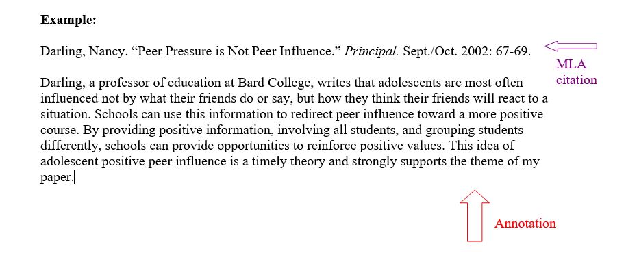
What to put in the annotation:

• Information: A summary of your findings
• Evaluation: What did you think of it, how will it help your topic
• Comparison: How it compares to other books/articles
• Authority: The background of the author

Annotated bibliographies are not difficult; just remember it’s an organized list of the sources you’ve used, each of which is followed by a brief note—the annotation.

Here are a couple of entries Antonio makes in his annotated bibliography for an essay he is writing on head injuries in football. Using the same search terms (“helmets,” “NFL,” and “head injuries”), a search of Academic Search Complete in his college library nets him entries 1, 2, and 4, and a search on Google nets him entry 3. Drawing from the color-coding suggestion, Antonio distinguishes between direct quotation (red), paraphrase (blue) and summary (purple), by using different font colors for each.

See below for another example of how your annotated bibliography can look in MLA format .

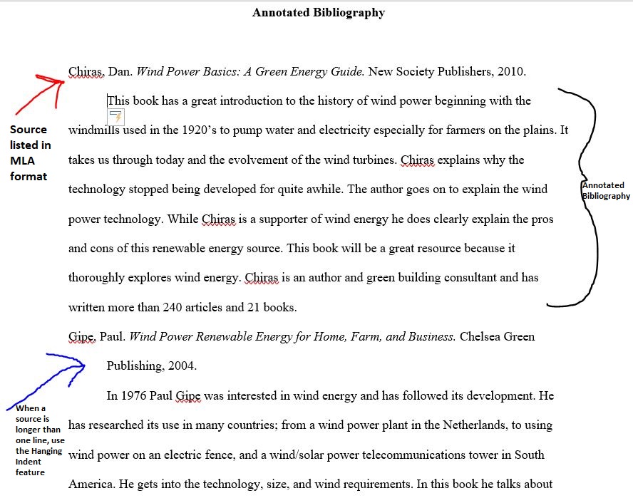
APA Annotated Bibliographies

The format above is similar for APA format — your annotated bibliography should be double-spaced; references should be in alphabetical order and have a hanging indent. However, your annotations should be fully indented as you would for a block quote. Here is an example:

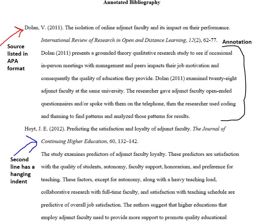
1. Choose a research topic of interest to you. Find a related website and find the following pieces of information: name of author, editor, or sponsoring organization; title of article; title of journal or site that has published the article; version or issue number; date of publication or access date.

2. Choose a research topic of interest to you. Find a related online blog.

3. Choose a research topic of interest to you and set up a related RSS feed.

4. Choose a research topic of interest to you. Find a related government site.

5. Choose a research topic of interest to you. Online, find a related photo, video, and table.

6. With your writing group sharing a couple of computers, amass several sources of an essay and write up an annotated bibliography.

7. Using Antonio’s essay idea on helmet hits in the NFL, draw up two statements of purpose that differ from each other in at least three of the six concerns (voice, audience, message, tone, attitude, or reception).

Attributions

• “Annotated Bibliography,” created by Dr. Sandi Van Lieu and licensed under CC BY NC SA 3.0 .
• Content from “ Chapter 7: Researching ” and licensed under CC BY NC SA .

The RoughWriter's Guide Copyright © 2020 by Dr. Sandi Van Lieu is licensed under a Creative Commons Attribution-NonCommercial-ShareAlike 4.0 International License , except where otherwise noted.

Share This Book

Purdue Online Writing Lab Purdue OWL® College of Liberal Arts

Annotated Bibliography Samples

Welcome to the Purdue OWL

This page is brought to you by the OWL at Purdue University. When printing this page, you must include the entire legal notice.

Copyright ©1995-2018 by The Writing Lab & The OWL at Purdue and Purdue University. All rights reserved. This material may not be published, reproduced, broadcast, rewritten, or redistributed without permission. Use of this site constitutes acceptance of our terms and conditions of fair use.

Below you will find sample annotations from annotated bibliographies, each with a different research project. Remember that the annotations you include in your own bibliography should reflect your research project and/or the guidelines of your assignment.

As mentioned elsewhere in this resource, depending on the purpose of your bibliography, some annotations may summarize, some may assess or evaluate a source, and some may reflect on the source’s possible uses for the project at hand. Some annotations may address all three of these steps. Consider the purpose of your annotated bibliography and/or your instructor’s directions when deciding how much information to include in your annotations.

Please keep in mind that all your text, including the write-up beneath the citation, must be indented so that the author's last name is the only text that is flush left.

Sample MLA Annotation

Lamott, Anne. Bird by Bird: Some Instructions on Writing and Life . Anchor Books, 1995.

Lamott's book offers honest advice on the nature of a writing life, complete with its insecurities and failures. Taking a humorous approach to the realities of being a writer, the chapters in Lamott's book are wry and anecdotal and offer advice on everything from plot development to jealousy, from perfectionism to struggling with one's own internal critic.

In the process, Lamott includes writing exercises designed to be both productive and fun. Lamott offers sane advice for those struggling with the anxieties of writing, but her main project seems to be offering the reader a reality check regarding writing, publishing, and struggling with one's own imperfect humanity in the process. Rather than a practical handbook to producing and/or publishing, this text is indispensable because of its honest perspective, its down-to-earth humor, and its encouraging approach.

Chapters in this text could easily be included in the curriculum for a writing class. Several of the chapters in Part 1 address the writing process and would serve to generate discussion on students' own drafting and revising processes. Some of the writing exercises would also be appropriate for generating classroom writing exercises. Students should find Lamott's style both engaging and enjoyable.

In the sample annotation above, the writer includes three paragraphs: a summary, an evaluation of the text, and a reflection on its applicability to his/her own research, respectively.

For information on formatting MLA citations, see our MLA 9th Edition (2021) Formatting and Style Guide .

Sample APA Annotation

Ehrenreich, B. (2001). Nickel and dimed: On (not) getting by in America . Henry Holt and Company.

In this book of nonfiction based on the journalist's experiential research, Ehrenreich attempts to ascertain whether it is currently possible for an individual to live on a minimum-wage in America. Taking jobs as a waitress, a maid in a cleaning service, and a Walmart sales employee, the author summarizes and reflects on her work, her relationships with fellow workers, and her financial struggles in each situation.

An experienced journalist, Ehrenreich is aware of the limitations of her experiment and the ethical implications of her experiential research tactics and reflects on these issues in the text. The author is forthcoming about her methods and supplements her experiences with scholarly research on her places of employment, the economy, and the rising cost of living in America. Ehrenreich’s project is timely, descriptive, and well-researched.

The annotation above both summarizes and assesses the book in the citation. The first paragraph provides a brief summary of the author's project in the book, covering the main points of the work. The second paragraph points out the project’s strengths and evaluates its methods and presentation. This particular annotation does not reflect on the source’s potential importance or usefulness for this person’s own research.

For information on formatting APA citations, see our APA Formatting and Style Guide .

Sample Chicago Manual of Style Annotation

Davidson, Hilda Ellis. Roles of the Northern Goddess . London: Routledge, 1998.

Davidson's book provides a thorough examination of the major roles filled by the numerous pagan goddesses of Northern Europe in everyday life, including their roles in hunting, agriculture, domestic arts like weaving, the household, and death. The author discusses relevant archaeological evidence, patterns of symbol and ritual, and previous research. The book includes a number of black and white photographs of relevant artifacts.

This annotation includes only one paragraph, a summary of the book. It provides a concise description of the project and the book's project and its major features.

For information on formatting Chicago Style citations, see our Chicago Manual of Style resources.