research paper on economics in india

Monetary policy framework in India

• Policy Review
• Published: 23 June 2020
• Volume 55 , pages 117–154, ( 2020 )

Cite this article

• Pami Dua 1  

47k Accesses

20 Citations

31 Altmetric

Explore all metrics

In 2016, the monetary policy framework moved towards flexible inflation targeting and a six member Monetary Policy Committee (MPC) was constituted for setting the policy rate. With this step towards modernization of the monetary policy process, India joined the set of countries that have adopted inflation targeting as their monetary policy framework. The Consumer Price Index (CPI combined) inflation target was set by the Government of India at 4% with ± 2% tolerance band for the period from August 5, 2016 to March 31, 2021. In this backdrop, the paper reviews the evolution of monetary policy frameworks in India since the mid-1980s. It also describes the monetary policy transmission process and its limitations in terms of lags and rigidities. It highlights the importance of unconventional monetary policy measures in supplementing conventional tools especially during the easing cycle. Further, it examines the voting pattern of the MPC in India and compares this with that of various developed and emerging economies. The synchronization of cuts in the policy rate by MPCs of various countries during the global slowdown in 2019 and the COVID-19 pandemic in the early 2020s is also analysed.

Similar content being viewed by others

Monetary Policy Framework in India

Monetary Policy: Global Trends and the Development of Bank of Russia’s Approaches

Inflation Targeting, Monetary Policy: The Way Forward

Avoid common mistakes on your manuscript.

1 Introduction

The monetary policy framework in India has evolved over the past few decades in response to financial developments and changing macroeconomic conditions. The operational framework of monetary policy has also gone through significant changes with respect to instruments and targeting mechanisms. The preamble of the Reserve Bank of India (RBI) Act, 1934 was also amended in 2016, which now clearly provides the mandate of the RBI. It reads as follows:

“to regulate the issue of Bank notes and keeping of reserves with a view to securing monetary stability in India and generally to operate the currency and credit system of the country to its advantage; to have a modern monetary policy framework to meet the challenge of an increasingly complex economy; to maintain price stability while keeping in mind the objective of growth.”

The aim of monetary policy in the initial years of inception of RBI was mainly to maintain the sterling parity, with exchange rate being the nominal anchor of monetary policy. Liquidity was regulated through open market operations (OMOs), bank rate and cash reserve ratio (CRR). Soon after independence and through the late 1960s, the role of the central bank was aligned with the planned development process of the nation in accordance with the 5-year plans. Thus, it played a major role in regulating credit availability, employing OMOs, bank rate, and reserve requirement towards this end.

With the nationalization of major banks in 1969, the main objective of monetary policy through the 1970s till the mid-1980s was the regulation of credit in accordance with the developmental needs of the country. This period was marked by monetization of fiscal deficit while inflationary consequences of high public expenditure necessitated frequent recourse to CRR.

In 1985, on the recommendation of the Committee set up to Review the Working of the Monetary System (Chairman: Dr. Sukhamoy Chakravarty), a new monetary policy framework, monetary targeting with feedback was implemented based on empirical evidence of a stable demand for money function. However, financial innovations in the 1990s implied that demand for money may be affected by factors other than income. Further, interest rates were deregulated in the mid-1990s and the Indian economy was getting increasingly integrated with the global economy. Therefore, the RBI began to deemphasize the role of monetary aggregates and implemented a multiple indicator approach (MIA) to monetary policy in 1998 encompassing all economic and financial variables that influence the major objectives outlined in the Preamble of the RBI Act. This was done in two phases—initially MIA and later augmented MIA (AMIA) which included forward looking variables and time series models.

Based on RBI’s Report of the Expert Committee to Revise and Strengthen the Monetary Policy Framework ( 2014 , Chairman: Dr Urjit R Patel), a formal transition was made in 2016 towards flexible inflation targeting and a six member Monetary Policy Committee (MPC) was constituted for setting the policy repo rate. The Monetary Policy Framework Agreement (MPFA) was signed between the Government of India and the RBI in February 2015 to formally adopt the flexible inflation targeting (FIT) framework. This was followed up with the amendment to the RBI Act, 1934 in May 2016 to provide a statutory basis for the implementation of the FIT framework. With this step towards modernization of the monetary policy process, India joined the set of countries that adopted inflation targeting, starting from 1990 by New Zealand, as their monetary policy framework. The Central Government notified in the Official Gazette dated August 5, 2016, that the Consumer Price Index (CPI) inflation target would be 4% with ± 2% tolerance band for the period from August 5, 2016 to March 31, 2021. At the time of writing (April 2020), this period is drawing to a close in less than a year. In this backdrop, this paper discusses the evolution of the monetary policy framework in India and describes the workings of the current framework.

The paper is divided into the following sections. Section  2 presents a schematic representation of the main components of a general monetary policy framework and describes its key features. Section  3 describes the genesis of the monetary policy framework in India since 1985 covering the Monetary Targeting Framework, Multiple Indicator Approach and Flexible Inflation Targeting. The main recommendations of RBI’s Report of the Expert Committee to Revise and Strengthen the Monetary Policy Framework ( 2014 , Chairman: Dr Urjit R Patel) are also discussed. Composition, workings and voting pattern of the Monetary Policy Committee from October 2016 to March 2020 are also provided. Further, a comparison of voting patterns with various countries across the globe is undertaken.

Section  4 discusses a general framework for monetary policy transmission and applies the framework to India. It also describes interest rate linkages at the global level. Section  5 examines unconventional monetary policy measures adopted in late 2019 and early 2020. Section  6 concludes the paper.

2 Schematic representation of a monetary policy framework

The specification of the monetary policy framework facilitates the conduct of monetary policy. The general framework comprises well-defined objectives/goals of monetary policy along with instruments, operating targets and intermediate targets that aid in the implementation of monetary policy and achievement of the ultimate objectives. A schematic representation of a monetary policy framework is shown in Fig.  1 (Laurens et al. 2015 ; Mishkin 2016 ).

Source: Author

Instruments are tools that the central bank has control over and are used to achieve the operational target. Examples of instruments include open market operations, reserve requirements, discount policy, lending to banks, policy rate. Operational targets are the financial variables that can be controlled by the central bank to a large extent through the monetary policy instruments and guide the day-to-day operations of the central bank. These can impact the intermediate target and thus help in the delivery of the final goal of monetary policy. Examples of operational targets include reserve money and short-term money market interest rates.

Intermediate targets are variables that are closely related with the final goals of monetary policy and can be affected by monetary policy. Intermediate targets may include monetary aggregates and short-term and long-term interest rates. Goals refer to the final policy objectives. These may include price stability, economic growth, financial stability and exchange rate stability.

This general framework is applied to the monetary targeting framework with feedback that prevailed from 1985 to 1998 and to the inflation targeting framework that exists from 2016 onwards. The multiple indicator approach that was operational from 1998 to 2016 was based on a number of financial and economic variables and was not exactly specified on the basis of this framework although broad money was treated as an intermediate target and the goals of monetary policy are the same across the various frameworks.

3 Genesis of monetary policy in India since 1985

3.1 monetary targeting with feedback: 1985–1998.

In the 1970s through the mid-1980s, monetization of the fiscal deficit exerted a dominant influence on monetary policy with inflationary consequences of high public expenditure necessitating frequent recourse to CRR. Against this backdrop, in 1985, on the recommendation of the Committee set up to Review the Working of the Monetary System (RBI 1985 ; Chairman: Dr. Sukhamoy Chakravarty), a new monetary policy framework, monetary targeting with feedback was implemented based on empirical evidence of a stable demand for money function. The recommendation of the committee was to control inflation within acceptable levels with desired output growth. Further, instead of following a fixed target for money supply growth, a range was followed which was subject to mid-year adjustments. This framework was termed “Monetary Targeting with Feedback” as it was flexible enough to accommodate changes in output growth.

This operational framework is depicted in Fig.  2 . (Definitions of variables shown in Fig.  2 are given in Appendix 1 ). The main instruments in this framework were cash reserve ratio (CRR), open market operations (OMOs), refinance facilities and foreign exchange operations. Broad money (M3) was chosen as the intermediate target while reserve money (M0) was the main operating target. However, an analysis of money growth outcomes during the monetary targeting framework reveals that targets were rarely met (RBI 2009–2012). Even with increases in CRR, money supply growth remained high and fuelled inflation.

(1) Primary objective of monetary policy in India is to maintain price stability, while keeping in mind the objective of growth.

(2) Definitions of variables are given in Appendix 1

Further, financial innovations in the 1990s implied that demand for money may be affected by factors other than income. Since the mid-1990s, with global integration, factors such as swings in capital flows, volatility in the exchange rate and global growth also impacted the economy. Moreover, interest rates were deregulated allowing for changing interest rates and a market determined management system of exchange rates was also adopted.

3.2 Multiple Indicator Approach: 1998–2016

Against the backdrop of changing domestic and global dynamics, RBI implemented a multiple indicator approach (MIA) to monetary policy in 1998 encompassing various economic and financial variables based on the recommendations of RBI’s Working Group on Money Supply (RBI 1998 ; Chairman: Dr YV Reddy). These variables included several quantity variables such as money, credit, output, trade, capital flows, fiscal indicators as well as rate variables such as interest rates, inflation rate and the exchange rate. The information on these variables provided a broad-based monetary policy formulation, which not only encompassed a diverse set of information, but also accorded flexibility to the conduct of monetary management. The MIA was conceptualized when Dr Bimal Jalan was Governor and was implemented in two stages—MIA and later augmented MIA, by including forward looking variables and a panel of time series models, in addition to the economic and financial variables (Mohanty 2010 ; Reddy 1999 ). Forward looking indicators were drawn from RBI’s industrial outlook survey, capacity utilization survey, inflation expectations survey and professional forecasters’ survey. All the variables together with time series models provided the projection of growth and inflation while RBI provided the projection for broad money (M3) and treated this as the intermediate target.

The operational framework of AMIA is illustrated in Fig.  3 . Compared to the Monetary Targeting Framework, the goals of monetary policy remained the same and broad money continued to serve as the intermediate target while the underlying operating mechanism of MIA evolved over time. In May 2011, the weighted average call money rate (WACR) was explicitly recognized as the operating target of monetary policy while the repo rate was made the only one independently varying policy rate. These measures improved the implementation and transmission of monetary policy along with enhancing the accuracy of signaling of monetary policy stance (Mohanty 2011 ).

Source: RBI Bulletin, December 2011

Shift towards inflation targeting

The importance of focusing on inflation was first highlighted in the Report of the Committee on Financial Sector Reforms (Government of India 2009 ; Chairman: Dr. Raghuram Rajan) constituted by the Government of India. The report recommended that RBI can best serve the cause of growth by focusing on controlling inflation and intervening in currency markets only to limit excessive volatility. The report pointed out that the cause of inclusion can also be best served by maintaining this focus because the poorer sections are least hedged against inflation. Further, the report recommended that there should be a single objective of staying close to a low inflation number, or within a range, in the medium term, moving steadily to a single instrument, the short-term interest rate to achieve it.

Former RBI Governor, Dr. Raghuram Rajan set up an Expert Committee in 2013 to Review and Strengthen the Monetary Policy Framework (RBI 2014 ; Chairman: Dr Urjit R Patel). The mandate of the Committee, amongst others, was to review the objectives and conduct of monetary policy in a globalized and highly inter-connected environment. The committee was also required to review the organizational structure, operating framework and instruments of monetary policy, liquidity management framework, to ensure compatibility with macroeconomic and financial stability, as well as market development. The impediments to monetary policy transmission were to be identified and measures along with institutional pre-conditions to improve transmission across financial markets and real economy were to be suggested.

Some issues central to the report were selecting the nominal anchor for monetary policy, defining the inflation metric and specifying the inflation target. A nominal anchor is central to a credible monetary policy framework as it ties down the price level or the change in the price level to attain the final goal of monetary policy. It is a numerical objective that is defined for a nominal variable to signal the commitment of monetary policy towards price stability.

Generally five types of nominal anchors have been used, namely, monetary aggregates, exchange rate, inflation rate, national income and price level. The Expert Committee recommended inflation to be the nominal anchor of the monetary policy framework in India as flexible inflation targeting recognizes the existence of growth-inflation trade-off in the short-run and stabilizing and anchoring inflation expectations is critical for ensuring price stability on an enduring basis. Further, low and stable inflation is a necessary precondition for sustainable high growth and inflation is also easily understood by the public.

Regarding the inflation metric, the Committee recommended that RBI should adopt the all India CPI (combined) inflation as the measure of the nominal anchor. This is to be defined in terms of headline CPI inflation, which closely reflects the cost of living and influences inflation expectations relative to other available metrics. CPI is also easily understood as it is used as a reference in wage contracts and negotiations. Headline inflation was preferred against core inflation (headline inflation excluding food and fuel inflation) since food and fuel comprise more than 50% of the consumption basket and cannot be discarded.

The Committee recommended the target level of inflation at 4% with a band of ± 2% around it. The tolerance band was formulated in the light of the vulnerability of the Indian economy to supply and external shocks and the relatively large weight of food in the CPI basket.

The Expert Committee also recommended that decision-making should be vested in a Monetary Policy Committee (MPC).

3.3 Flexible inflation targeting: 2016 onwards

With the signing of the Monetary Policy Framework Agreement (MPFA) between the Government of India and the RBI on Feb 20, 2015, Flexible Inflation Targeting (FIT) was formally adopted in India. In May 2016, the Reserve Bank of India (RBI) Act, 1934 was amended to provide a statutory basis for the implementation of the FIT framework. The amended RBI Act, 1934 also provided that the Central Government shall, in consultation with the Bank, determine the inflation target in terms of the Consumer Price Index, once in every 5 years.

Accordingly, the Central Government has notified in the Official Gazette 4% Consumer Price Index (CPI) inflation as the target for the period from August 5, 2016 to March 31, 2021 with the upper tolerance limit of 6% and the lower tolerance limit of 2%. The amended RBI Act, 1934 also provides that RBI shall be seen to have failed to meet the target if inflation remains above 6% or below 2% for three consecutive quarters. In such circumstances, RBI is required to provide the reasons for the failure, and propose remedial measures and the expected time to return inflation to the target.

In 2016, India thus joined several developed and emerging market economies that have implemented inflation targeting. Figure  4 shows the timeline for implementation of inflation targeting for countries in this category, starting in 1990.

Source: Centre for Central Banking Studies (2012), Bank for International Settlements (2017), Russian Journal of Economics (2017), The Economist (2016), Central Bank websites of Kazakhstan and Ukraine

Monetary Policy Committee: composition, monetary policy framework and voting patterns

The amended RBI Act, 1934 provides for a statutory and institutionalized framework for a six-member Monetary Policy Committee (MPC) to be constituted by the Central Government by notification in the Official Gazette. The Central Government in September 2016 thus constituted the MPC with three members from RBI including the Governor as Chairperson and three external members as per Gazette Notification dated September 29, 2016. (Details of the composition of MPC are given in Appendix 3 ). The Committee is required to meet at least four times a year although it has been meeting on a bi-monthly basis since October 2016. Each member of the MPC has one vote, and in the event of equality of votes, the Governor has a second or casting vote. The resolution adopted by the MPC is published after conclusion of every meeting of the MPC. On the 14th day, the minutes of the proceedings of the MPC are published which includes the resolution adopted by the MPC, the vote of each member on the resolution, and the statement of each member on the resolution.

It may be noted that before the constitution of the MPC, a Technical Advisory Committee (TAC) on Monetary Policy was set up in 2005 which consisted of external experts from monetary economics, central banking, financial markets and public finance. The role of this committee was to enhance the consultative process of monetary policy by reviewing the macroeconomic and monetary developments in the economy and advising RBI on the stance of monetary policy. With the formation of MPC, the TAC on Monetary Policy ceased to exist.

The MPC is entrusted with the task of fixing the benchmark policy rate (repo rate) required to contain inflation within the specified tolerance band. The framework entails setting the policy rate on the basis of current and evolving macroeconomic conditions. Once the repo rate is announced, the operating framework looks at liquidity management on a day-to-day basis with the aim to anchor the operating target—the weighted average call rate (WACR)—around the repo rate. This is illustrated in Fig.  5 , where the intermediate targets are the short-term and long-term interest rates and the goals of price stability and economic growth are aligned with the primary objective of monetary policy to maintain price stability, keeping in mind the objective of growth. In addition to the repo rate, the instruments include liquidity facility, CRR, OMOs, lending to banks and foreign exchange operations (RBI 2018 ).

It is imperative here to note some of the key elements of the revised framework for liquidity management (RBI 2019 ) that are particularly relevant for the operating framework shown in Fig.  5 . As noted in the RBI Monetary Policy Report, 2020.

Liquidity management remains the operating procedure of monetary policy; the weighted average call rate (WACR) continues to be its operating target.

The liquidity management corridor is retained, with the marginal standing facility (MSF) rate as its upper bound (ceiling) and the fixed reverse repo rate as the lower bound (floor), with the policy repo rate in the middle of the corridor.

The width of the corridor is retained at 50 basis points—the reverse repo rate being 25 basis points below the repo rate and the MSF rate 25 basis points above the repo rate. (The corridor width was asymmetrically widened on March 27 and April 17, 2020.)

Instruments of liquidity management continue to include fixed and variable rate repo/reverse repo auctions, outright open market operations, forex swaps and other instruments as may be deployed from time to time to ensure that the system has adequate liquidity at all times.

The current requirement of maintaining a minimum of 90% of the prescribed CRR on a daily basis will continue. (This was reduced to 80% on March 27, 2020.)

The first meeting of the MPC was held in October 2016. Between October 2016 and March 2020, the MPC has met 22 times. Table 1 shows the voting patterns for each meeting with respect to the direction of change in the policy rate, magnitude of change and the stance of monetary policy. Table 2 , on the other hand, provides an overall summary of the voting of all the meetings. It is interesting to note in Table 2 , that with respect to direction of change/status quo of the policy rate, consensus was achieved in 12 meetings out of 22. Of these 12 meetings, there were three meetings where there were differences in the magnitude of the change voted for although there was consensus regarding the direction of change. The diversity in voting of the MPC members reflects the differences in the assessment and expectations of individual members as well as their policy preferences.

To examine if this diversity exists in MPCs of other countries as well, we analyse the voting patterns of 18 countries across the globe during October 2018 to March 2020 in Table 3 . For many countries, we find dissents in some of the meetings, similar to the lack of consensus in some of the meetings of the Indian MPC.

It merits mention that the committee approach towards the conduct of monetary policy has gained prominence across globe. The advantages of this approach include confluence of specialized knowledge and expertise on the subject domain, bringing together different stakeholders and diverse opinions, improving representativeness and collective wisdom, thus making the whole greater than the sum of parts (Blinder and Morgan 2005 ; Maier 2010 ). Further, Rajan ( 2017 ) notes that MPC would bring more minds to bear on policy setting, preserve continuity in case a member has to quit or retire, and be less subject to political pressures.

4 Monetary policy transmission framework

This section presents a stylized representation of a framework for monetary policy transmission and also applies this framework to India.

Monetary policy transmission is the process through which changes in monetary policy affect economic activity in general as well as the price level. With developments in financial systems, the world over, and growing sophistication of financial markets, most central banks use the short-term interest rate as the policy instrument for the conduct of monetary policy. Monetary policy transmission is thus the process through which a change in the policy rate is transmitted first to the short-term money market rate and then to the entire maturity spectrum of interest rates covering the money and bond markets as well as banks’ deposit and lending rates. These impulses, in turn, impact consumption (private and government), investment and net exports, which affect aggregate demand and hence output and inflation.

There are five channels of monetary transmission—interest rate channel; exchange rate channel; asset price channel; credit channel and expectations channel. The interest rate channel is described above. Monetary transmission takes place through the exchange rate channel when changes in monetary policy impact the interest rate differential between domestic and foreign rates leading to capital flows (inflow or outflow) which in turn affects the exchange rate and hence the relative demand for exports and imports. Transmission through the asset price channel occurs when changes in monetary policy influence the price of assets such as equity and real estate that lead to changes in consumption and investment. A change in prices of assets can lead to a change in consumption spending due to the associated wealth effect. For example, if interest rates fall, people may consider purchasing assets that are non-interest bearing such as real estate and equity. A rise in demand for these assets may result in higher prices, a positive wealth effect and thus higher consumption. Further if equity prices rise, firms may increase investment spending. Transmission through the credit channel happens if monetary policy influences the quantity of available credit. This may happen if the willingness of financial institutions to lend changes due to a change in monetary policy. Further, debt obligations of businesses may also change due to a change in the interest rate. For instance, if the policy rate falls, debt obligations of firms may decrease, strengthening their balance sheets. As a result, financial institutions may be more willing to lend to businesses, thus increasing investment spending. Monetary policy changes can impact public’s expectations of output and inflation and accordingly, aggregate demand can be impacted via the expectations channel . For instance, expected future changes in the policy rate can impact medium-term and long-term expected interest rates through market expectations and thus affect aggregate demand. Further, if inflation expectations are firmly anchored by the central bank, this would imply price stability.

A stylized representation of the monetary policy transmission framework of a change in the policy rate is shown in Fig.  6 . Figure  7 depicts the monetary transmission through the interest rate channel with specific reference to India. (Definitions of all variables shown in Fig.  6 are given in Appendix 2 .) This shows that a change in the policy rate (repo rate) first impacts the call money rate (weighted average call money rate—WACR) and in turn all other money market rates as well as bond market rates including the repo market, certificates of deposit (CD) and commercial paper (CP) markets, Treasury Bill (T-Bill) market, Government Securities (G-Sec) market and the Bond Market. The lending rate of banks also changes as depicted by the marginal cost of funds based lending rate (MCLR). This further impacts consumption and investment decisions as well as net exports and through these, aggregate demand and ultimately the goals of monetary policy. Details of the monetary transmission process are given in RBI ( 2020c ).

(1) Definitions of variables are given in Appendix 2

The transmission mechanism is beset with lags. As explained in simple terms in Rangarajan ( 2020 ), there are two components of the transmission mechanism. The first is how far the signals sent out by the central bank are picked by the banks and the second is how far the signals sent out by the banking system impact the real economy. Rangarajan ( 2020 ) labels the first component as “inner leg” and the second as “outer leg”.

To illustrate monetary transmission of the first kind, we examine the impact of a cumulative reduction in the policy repo rate by 135 basis points between February 2019 and January 2020. During this period, transmission to various money and bond markets ranged from 146 basis points in the overnight call money market to 73 basis points in the market for 5-year government securities to 76 basis points in the market for 10-year government securities. Transmission to the credit market was also modest with the 1-year median marginal cost of funds-based lending rate (MCLR) declining by 55 basis points during February 2019 and January 2020. The weighted average lending rate (WALR) on fresh rupee loans sanctioned by banks fell by 69 basis points while the WALR on outstanding rupee loans declined by 13 basis points during February to December 2019.

Monetary transmission increased somewhat after the introduction of the external benchmark system in October 2019 whereby most banks have linked their lending rates to the policy repo rate of the Reserve Bank. During October to December 2019, the WALRs of domestic banks on fresh rupee loans fell by 18 basis points for housing loans, 87 basis points for vehicle loans and 23 basis points for loans to micro, small and medium enterprises (MSMEs).

Monetary transmission in various markets is depicted in Figs. 8 , 9 and 10 . Figure  8 shows the policy corridor with the MSF rate as the ceiling and the reverse repo rate as the floor for the daily movement in the weighted average call money rate. The figure shows that the WACR moved closely in tandem with the policy rate (repo rate). Figure  9 shows that the G-Sec market rates followed the movements in the policy rate. Figure  10 shows that the direction of change of MCLR was more or less in synchronization with that of the repo rate. The WALR for fresh rupee loans tracked the repo rate much more than the WALR on outstanding loans.

Source: RBI Database on Indian Economy, RBI Weekly Statistical Supplement

Source: RBI Database on Indian Economy

Source: RBI Website

Figure  11 shows the 4% target inflation rate with the ± 2% tolerance band along with the headline inflation rate. This shows that the headline inflation generally stayed within the band. The average inflation rate from August 2016 to March 2020 was 3.93% and up to December 2019, it was 3.72%, i.e. close to 4%. The average GDP growth between Q2: 2016–2017 and Q3: 2019–2020 was 6.6% (Fig.  12 ).

Source: Ministry of Statistics and Programme Implementation, GOI

An interesting phenomena, world-wide is the synchronization in the movements in interest rates across the globe. Table 4 shows that MPCs in various countries have voted for a cut in their policy rate in 2019 at a time when many countries were simultaneously experiencing a slowdown. Due to COVID-19 pandemic, in early 2020, some countries have cut the policy rate sharply. This pattern of rate cuts in 2019 up to March 2020 is almost perfectly aligned with the movements in the repo rate (policy rate) in India. These global patterns are illustrated in Figs.  13 and 14 . Figure  13 shows that the policy rates for the BRICS nations moved in tandem from 2017 to 2020. Figure  14 indicates a similar pattern amongst policy rates of US, ECB, UK and Japan.

Source: Central Bank Websites. Brazil: Selic Rate; Russia: Key Rate; India: Repo Rate; China: Interest Rate; South Africa: Repo Rate

Source: Central Bank Websites. US: Fed Funds Rate; ECB: Interest Rate on the Deposit Facility; UK: Bank Rate; Japan: Policy Interest Rate

5 Unconventional monetary policy measures

We have so far discussed conventional monetary policy. As already described, monetary transmission of conventional monetary policy entails a change in the policy rate impacting financial markets from short-term interest rates to longer-term bonds and bank funding and lending rates. A change in the policy rate is thus expected to permeate through the entire spectrum of rates that further translates into affecting interest sensitive spending and thus economic activity. However, if there are problems in the monetary policy transmission mechanism or if additional monetary stimulus is required in the circumstances that the policy rate cannot be reduced further (or in addition to a change in the policy rate), then the central banks may employ unconventional monetary policy tools. Unconventional monetary measures target financial variables other than the short-term interest rate such as term spreads (e.g., interest rates on risk free bonds), liquidity, credit spreads (e.g. interest rates on risky assets) and asset prices. The objective of unconventional tools is to supplement the conventional monetary policy tools especially in the easing cycle to boost economic growth.

In the recent past, RBI has utilized various unconventional tools in addition to conventional monetary policy measures. To better understand the use of unconventional tools in the Indian economy, examples of unconventional monetary policy tools are first analysed and their applications to the Indian scenario are described. Broadly, unconventional measures can be classified into four categories—large scale asset purchases, lending operations, forward guidance and negative interest rates (BIS 2019 ). The key features of the measures and their applications in India are described in Table 5 .

Large scale asset purchases (also referred to as quantitative easing) by a central bank involve purchase of long-term government securities financed by crediting reserve accounts that commercial banks hold at the central bank. This purchase would lower government bond yields and serve as a signal that the policy rate will stay at a lower level for a longer period. Sellers of government bonds may, in turn, change their investment portfolios and invest in more risky assets (e.g., corporate bonds) leading to a decrease in the relevant interest rate and higher asset price and thus boost economic growth. Central banks can also purchase assets from the private sector.

Lending operations entail provision of liquidity to financial institutions by the central bank through the creation of new or extension of existing lending facilities. This mechanism is different from conventional lending since this is undertaken at looser or specific conditions, e.g., expanding the set of eligible collateral, extending maturity of the loan, providing funding at lower cost and channel/target lending to desired areas or activities with explicit conditions on loans. This lending increases the credit flows to the private sector and helps to restart flow of credit to credit-starved sectors. It can also lead to lower borrowing costs for the financial and real economy sectors.

Forward guidance involves central banks communicating future policy intentions and commitments regarding the policy rate to influence policy expectations. Forward guidance is given routinely by most central banks. Its use as an unconventional tool implies that a central bank uses this to signal that it is open to undertaking extraordinary policy actions for a longer duration. Forward guidance can be ‘time specific’ or ‘state specific’. Under the former, the central bank makes a commitment to keep interest rates low for a specified period. Under the latter, the central bank maintains low rates until specific economic conditions are met.

The rationale of a negative interest rate is that if an interest rate is charged on the reserves that commercial banks hold at the central bank, the banks may be induced to reduce their excess reserves by increasing lending.

The first three of these have been applied to India and are reported in Table 4 . These include Operations Twist in December 2019 and January as well as April 2020, long-term repo operation (LTRO) in February 2020, targeted long-term repo operations (TLTRO) in March and April 2020, and special refinance facilities to National Bank for Agriculture and Rural Development (NABARD), Small Industries Development Bank of India (SIDBI) and National Housing Bank (NHB) in April 2020.

The application of these unconventional monetary tools was necessitated, first by the slowdown in the Indian economy in 2019, and second, by the impact of COVID-19 pandemic due to which economic activity and financial markets, the world over, came under severe stress. It was thus necessary for the Reserve Bank to employ measures to mitigate the impact of COVID-19, revive growth and preserve financial stability. Thus the unconventional monetary policy tools supplemented the conventional monetary policy measures to stimulate growth in the economy.

6 Conclusions

This paper reviews the evolution of monetary policy frameworks in India since the mid-1980s. It also describes the monetary policy transmission process and its limitations in terms of lags in transmission as well as the rigidities in the process. It also highlights the importance of unconventional monetary policy measures in supplementing conventional tools especially during the easing cycle.

At the time of writing (April 2020), three and a half years have passed since the implementation of the Flexible Inflation Targeting Framework and the constitution of the Monetary Policy Committee. With the implementation of FIT, India joined the group of various developed, emerging and developing countries that have implemented inflation targeting since 1990.

The inflation target specified by the Central Government was 4% for the Consumer Price Index (CPI) inflation for the period from August 5, 2016 to March 31, 2021 with the upper tolerance limit of 6% and the lower tolerance bound of 2%. As shown in Fig.  11 , from August 2016 through March 2020, the headline inflation generally stayed within the tolerance band with the average inflation rate slightly less than 4% during this period. There were episodes of high/unusual inflation due to supply shocks (food inflation, oil prices) but these were suitably integrated in the policy decisions.

The Monetary Policy Committee has also been in existence since October 2016. The mandate of the MPC is to set the policy repo rate while taking cognizance of the primary objective of monetary policy—to maintain price stability while keeping in mind the objective of growth—as well as the target inflation rate within the tolerance band. Once the policy repo rate is set, the monetary transmission process facilitates the percolation of the change in the policy rate to all financial markets (money and bond markets) as well as the banking sector which further impacts interest sensitive spending in the economy and eventually increases aggregate demand and output growth.

In practice, however, there are rigidities as well as lags in the transmission process that impede the speed and magnitude of the transmission and thus question the efficacy of monetary policy with respect to the policy repo rate. Nevertheless, the external benchmarking system introduced by RBI from October 1, 2019 whereby all new floating rate personal or retail loans (housing, auto etc.) and floating rate loans to micro and small enterprises extended by banks were benchmarked to an external rate, strengthened the monetary transmission process with several banks benchmarking their lending rate to the policy repo rate. This requirement of an external benchmark system was further expanded to cover new floating loans to Medium Enterprises extended by banks with effect from April 1, 2020. This is expected to further improve the transmission process.

Of course, the policy repo rate is not a panacea for all ills but serves well as a signaling rate. The RBI routinely brings out the Statement on Developmental and Regulatory Policies Footnote 1 that is released simultaneously with the resolution of the MPC. RBI has also taken recourse to unconventional measures to supplement the conventional tools to boost economic growth. More recently, with the slowdown in 2019 followed by the extraordinary slump in economic activity due to COVID-19 pandemic, RBI has been compelled to use rather innovative and unconventional tools starting in December 2019 as discussed in Table 5 .

Needless to say, in the unprecedented times of the global pandemic (and, in general, in periods of severe crises), a multi-pronged approach comprising monetary, fiscal and other policy measures is required to protect economic activity and minimize the negative impact of the pandemic (crisis) on economic growth. The importance of monetary-fiscal coordination is highlighted in the resolution of the Monetary Policy Committee dated March 27, 2020 (available on the RBI website) that states the following: “Strong fiscal measures are critical to deal with the situation.” Thus, in addition to monetary policy, fiscal policy has a major role in combating the economic effects of the COVID-19 pandemic. In response to the need of the hour, the Government of India has implemented various fiscal measures to provide a boost to the economy. While central banks across the globe have responded to the global pandemic with monetary and regulatory measures, various governments have reinforced the monetary measures by deploying massive fiscal measures to shield economic activity from the effect of the COVID-19 pandemic.

A few words about the workings of the MPC are also warranted. As discussed in the paper, the voting pattern of the Indian MPC is comparable to international standards, reflecting the healthy diversity in the assessment of the members. The workings of the MPC are transparent with the resolution being made available soon after the end of the meetings. Furthermore, each member of the Committee has to submit a statement that is made available in the public domain on the 14th day after the meeting. Thus, each member is individually accountable, making the process perhaps more stringent than that of MPCs in other countries.

Statement on Developmental and Regulatory Policies sets out various developmental and regulatory policy measures and macroprudential policies for strengthening financial markets and systems, regulation and supervision, banking sector etc. from time to time.

Interest rates on fixed rate loans of tenor below 3 years shall not be less than the benchmark rate for similar tenor.

In case of newly set up banks (either domestic or foreign banks operating as branches in India) where lending operations are mainly financed by capital, the weightage for this component may be higher in proportion to the extent of capital deployed for lending. This dispensation will be available for a period of three years from the date of commencing operations.

Bank for International Settlements. (2019). Unconventional monetary policy tools: a cross-country analysis. Report by a Working Group (Chaired by: Simon M. Potter, Federal Reserve Bank of New York and Frank Smets, European Central Bank). Committee on the Global Financial System. BIS.

Blinder, A., & Morgan, J. (2005). Are two heads better than one? An experimental analysis of group versus individual decision-making. Journal of Money, Credit and Banking, 35 (5), 789–811.

Google Scholar  

Government of India. (2009). A hundred small steps: Report of the committee on financial sector reforms (Chairman: Raghuram Rajan) . New Delhi: Planning Commission.

Hammond, G. (2012). State of the art of inflation targeting. Handbooks, Centre for Central Banking Studies, Bank of England, 4th edn, number 29

Hattori, M., Yetman, J. (2017). The evolution of inflation expectations in Japan. Bank of International Settlements Working Papers, No. 647. Bank of International Settlements, pp 1–3

Korhonen, L., & Nuutilainen, R. (2017). Breaking monetary policy rules in Russia. Russian Journal of Economics, 3 (4), 366–378.

Article   Google Scholar  

Laurens, B.J., Eckhold, K., King, D., Maehle, N., Naseer, A., Durré, A. (2015). The journey of inflation targeting: Easier said than done the case for transitional arrangements along the road. International Monetary Fund, WP/15/136.

Maier, P. (2010). How central banks take decisions: an analysis of monetary policy meetings. In P. L. Siklos, M. T. Bohl, & M. E. Woher (Eds.), Challenges in central banking: the current institutional environment and forces affecting monetary policy . Cambridge: Cambridge University Press.

Mishkin, F. S. (2016). The economics of money, banking, and financial markets . Pearson: Columbia University.

Mohanty, D. (2010). Monetary policy framework in India: Experience with multiple-indicators approach. In: Speech delivered at the Conference of the Orissa Economic Association in Baripada, Orissa on 21st February, 2010. Orissa

Mohanty, D. (2011). Changing contours of monetary policy in India . Mumbai: Reserve Bank of India Bulletin. (Dec 2011)

Rajan, R. G. (2017). I do what I do . New Delhi: Harper Collins.

Rangarajan, C. (2020). The new monetary policy framework—What it means. In: Prof. Sukhamoy Chakravarty Memorial Lecture, delivered at Annual Conference of the Indian Econometric Society at Madurai Kamaraj University in January 2020 . https://www.nipfp.org.in/media/medialibrary/2020/02/WP_297_2020.pdf

Reddy, Y.V. (1999) Monetary policy operating procedures in India. In: Bank of International Settlements. (Ed.) Monetary policy operating procedures in emerging market economies. BIS Policy Papers No. 5 , pp 99–109

Reserve Bank of India. (1985). Report of the committee to review the working of the monetary system (Chairman: Dr. Sukhamoy Chakravarty). Mumbai

Reserve Bank of India. (1998). Report of the working group on money supply: analytics and methodology of compilation (Chairman: Dr. Y. V. Reddy). Mumbai.

Reserve Bank of India. (2013). Report on currency and finance 2009–2012: fiscal-monetary co-ordination. Mumbai.

Reserve Bank of India. (2014). Report of the expert committee to revise and strengthen the monetary policy framework (Chairman: Dr. Urjit Patel). Mumbai.

Reserve Bank of India. (2017). Report of the internal study group to review the working of the marginal cost of funds based lending rate system (Chairman: Dr. Janak Raj). Mumbai.

Reserve Bank of India. (2018). Forex market operations and liquidity management (by—Janak Raj, Sitikantha Pattanaik, Indranil Bhattacharya and Abhilasha) . Mumbai: Reserve Bank of India Bulletin.

Reserve Bank of India. (2019). Report of the internal working group to review the liquidity management framework. Mumbai.

Reserve Bank of India. (2020a). Governor’s statement, sixth bi-monthly monetary policy statement, February 6, 2020. Mumbai.

Reserve Bank of India. (2020b). Governor’s statement, seventh bi-monthly monetary policy statement, March 27, 2020. Mumbai.

Reserve Bank of India. (2020c). Monetary policy transmission in India—Recent trends and impediments (by—Arghya Kusum Mitra and Sadhan Kumar Chattopadhyay). Reserve Bank of India Bulletin, March. Mumbai.

Reserve Bank of India. (2020d). Monetary Policy Report, April. Mumbai.

Reserve Bank of India. (2020e). Governor’s Statement, April 17, 2020. Mumbai.

The Economist Intelligence Unit. (2016). Argentine Central Bank adopts inflation-targeting regime. Financial Services, The Economist Group, September.

Vasudevan, A. (2017). Reflections on analytical issues in monetary policy: The Indian Economic Realities. Economic and Political Weekly, 52 (12), 45–52.

Download references

Acknowledgements

I am grateful to Michael Patra and Janak Raj, Deputy Governor and Executive Director respectively, Reserve Bank of India for useful and constructive suggestions. I also gratefully acknowledge help and support from Hema Kapur, Deepika Goel and Neha Verma, teachers in colleges of the University of Delhi, who also motivated me to write in a student-friendly manner. Special thanks are due to Naina Prasad for competent and diligent research assistance. I am grateful to the Editors of the Indian Economic Review for inviting me to contribute to the newly instituted section on Policy Review. Earlier versions of this paper were presented as a Public Lecture at the Delhi School of Economics in March 2020 and as a Keynote Address at the Annual Conference of the Indian Econometric Society at Madurai Kamaraj University in January 2020. I am grateful to the participants of these events for their feedback.

Author information

Authors and affiliations.

Department of Economics, Delhi School of Economics, University of Delhi, Delhi, India

You can also search for this author in PubMed   Google Scholar

Corresponding author

Correspondence to Pami Dua .

Additional information

Publisher's note.

Springer Nature remains neutral with regard to jurisdictional claims in published maps and institutional affiliations.

The views expressed in this paper are of the author and not of the Monetary Policy Committee (MPC), of which she is a member.

Appendix 1: Glossary (Figs. 2 and 5 )

Source: Handbook on RBI’s Weekly Statistical Supplement; Reserve Bank of India Website

Appendix 2: Glossary (Fig. 8 )

Appendix 3: constitution of the monetary policy committee.

The Gazette Notification of the Ministry of Finance dated September 29, 2016 notes the following.

“In exercise of the powers conferred by Section 45ZB of the Reserve Bank of India Act, 1934 (2 of 1934), the Central Government hereby constitutes the Monetary Policy Committee of the Reserve Bank of India, consisting of the following, namely:

The Governor of the Bank—Chairperson, ex officio;

Deputy Governor of the Bank, in charge of Monetary Policy—Member, ex officio;

One officer of the Bank to be nominated by the Central Board—Member, ex officio;

Shri Chetan Ghate, Professor, Indian Statistical Institute (ISI)—Member;

Professor Pami Dua, Director, Delhi School of Economics (DSE)—Member; and

Dr. Ravindra H. Dholakia, Professor, Indian Institute of Management, Ahmedabad, Member.”

The three external members have served on the Committee since its inception and continue to serve. There have been some changes in the RBI members as follows.

Former Governor, Dr. Urjit Patel chaired the Committee from October 2016 to December 2018. Governor, Shri Shaktikanta Das presided from the February 2019 meeting onwards.

Shri R. Gandhi, Former Deputy Governor attended the October and December meetings in 2016.

Dr. Viral Acharya, Former Deputy Governor in charge of Monetary Policy attended the meetings from February 2017 to June 2019.

Shri Bibhu Prasad Kanungo, Deputy Governor attended the meetings from August to December 2019.

Dr, Michael Patra attended all the meetings, first as Executive Director till December 2019 and continues to attend meetings as Deputy Governor in charge of Monetary Policy.

Dr. Janak Raj has attended meetings since February 2020 as Executive Director.

Rights and permissions

Reprints and permissions

About this article

Dua, P. Monetary policy framework in India. Ind. Econ. Rev. 55 , 117–154 (2020). https://doi.org/10.1007/s41775-020-00085-3

Download citation

Published : 23 June 2020

Issue Date : June 2020

DOI : https://doi.org/10.1007/s41775-020-00085-3

Share this article

Anyone you share the following link with will be able to read this content:

Sorry, a shareable link is not currently available for this article.

Provided by the Springer Nature SharedIt content-sharing initiative

• Inflation targeting
• Monetary Policy Committee
• Monetary transmission process
• Unconventional monetary policy measures

JEL Classification

• Find a journal
• Publish with us
• Track your research

The Official Journal of the Pan-Pacific Association of Input-Output Studies (PAPAIOS)

• Open access
• Published: 09 May 2020

Tax structure and economic growth: a study of selected Indian states

• Yadawananda Neog   ORCID: orcid.org/0000-0002-3578-0460 1 &
• Achal Kumar Gaur 1  

Journal of Economic Structures volume  9 , Article number:  38 ( 2020 ) Cite this article

49k Accesses

27 Citations

3 Altmetric

Metrics details

The present study examines the long-run and short-run relationship between tax structure and state-level growth performance in India for the period 1991–2016. The analysis in this paper is based on the model of Acosta-Ormaechea and Yoo ( 2012 ), and for the verification of the relationship between taxation and economic growth the panel regression method is used. With the use of 14 Indian states data, Panel Pool mean group estimation indicates that income tax and commodity–service tax have negative effects whilst property and capital transaction tax have a significant positive effect on state economic growth. This study finds ‘U’ shape relationship between tax structure and growth performance. Based on the analysis, we conclude that for faster growth of Indian states, policymakers should give more focus on property taxes along with the reduction in income taxes.

1 Introduction

The study on the potential association between tax structure and growth performance has gathered a great deal of attention from policymakers, academicians and regulatory circles for several reasons. First, the developing and emerging economies require a large volume of tax revenues for the smooth and efficient functioning of the state at both the national and sub-national levels. Globalization has laid down the foundation for Goods and Service Tax (GST) in many developing countries (Mcnabb 2018 ). Due to competition, developing countries are also facing the difficulties to maintain existing tax revenues (Bird and Zolt 2011 ). Second, tax collection and structure of it create distortionary impacts in the economy through tax burden. Thus, the positive and negative impact of tax made the ‘tax–growth’ relationship more complex and the structure of taxation has a definite role in the development process of an economy.

In a budget constraint economy like India, investigation of tax–growth relationship enables us to formulate the suitable policy measure for the more inclusive and equitable growth process. The budget crisis is usually resolved through the cut-down of public spending or/and an increase in tax revenues (Macek 2014 ). Rapid reduction in spending or increase in taxes is harmful to long-run growth performance. Thus, the concern of the government lies with the problem of fiscal consolidation with sustainable growth performance where tax policies are vital.

Empirical evidence on the impact of tax structure on growth performance is not conclusive. India has adopted the Goods and Service Tax (GST) policy in 2017 intending to raise indirect tax collections and transform the indirect tax structure into a single market to avoid tax evasions and double taxation. GST is regarded as one of the major tax policy changes in independent India and economists are an optimist about its impact on revenue generations and growth performance. But this policy is not the only policy that shaped in independent India; other major policy changes also take place after independence. Footnote 1 Tax Reform Committee (TRC) report of 1991 regarded one of the productive and structured policy recommendations in the recent decade. At the state level, sales tax reform in the form of Value Added Tax (VAT) in 2005 becomes a fruitful policy initiative. However, the tax collections in both national and sub-national level are still low as compared to the international standards. Changes in tax policy also change in the tax structure in the economy and India witnessed these changes at both levels of governments. Recent studies proved that the changes in tax structure have decisive implication in the growth performance through work–leisure behaviour, investment decisions and overall productivity (Arnold et al. 2011 ; Gemmell et al. 2011 ; Macek 2014 ; Mdanat et al. 2018 ; Durusu-Ciftci 2018 ). In India, very few empirical studies are available which analyse the impact of these changes in tax structure on growth performance and this study will be first to investigate tax–growth nexus in India with the use of state-level data.

This analysis primarily concerned with tax structure rather than to tax levels (usually measured as a tax–GDP ratio). The main advantage of tax structure analysis is that it provides revenue-neutral tax policy changes which remove the difficulties related with the question of how aggregate tax revenue changes relates with expenditure changes (Arnold et al. 2011 ). The empirical results from linear panel regression suggest us that property and capital transection tax are positively affecting the state’s growth performance, where commodity and service tax effect negatively. However, the non-linear panel regression indicates that the positive effect is only visible for property taxes at a higher level where the negative effect of commodity and service taxes becomes positive after a threshold point. The effect of income tax is not significant in long run irrespective of panel regression models.

The structure of the paper is as follows: Sect.  2 deals with the theoretical framework and empirical literature, followed by a brief description of data and methodology in Sect.  3 . Empirical results and discussion are presented in Sect.  4 and our last Sect.  5 is for conclusions and recommendations.

2 Theoretical framework and empirical literature

Growth literature very recently acknowledges the role of taxation in the growth process of an economy. Until recently, growth models are more concerned with the steady-state process and exogenous changes. On the theoretical ground, taxation does not have any impact on growth (Myles 2000 ). Development of endogenous growth models creates the space for fiscal policy especially tax policy in determining the growth performance. Barro ( 1990 ), King and Rebello ( 1990 ) and Jones et al. ( 1993 ) were the pioneer in this regard. Tax level and tax structure have an impact on the saving behaviour of the household and investment in human capital. On the other hand, the firm also changes its investment decisions and innovations following tax policies (Johansson et al. 2008 ). These decisions and incentives in the accumulation of physical and human capital create the ‘Growth’ disparities amongst the countries and state economies.

A large body of literature available on “Tax-Growth” relationship is mostly dedicated to cross-country settings (Martin and Fardmanesh 1990 ; Karras 1999 ; Myles 2000 ; Tosun and Abizadeh 2005 ; Johansson et al. 2008 ; Vartia et al. 2008 ; Arnold 2011 ; Szarowska 2013; Macek 2014 ; Stoilova 2017 ; Safi et al. 2017 ; Durusu-Ciftci 2018 ) that investigates the effect of tax policy on economic performance. Income and corporation taxes are the major tax instruments for the governments irrespective of the level of developments of a country. The formation of tax structure with these two taxes has many implications in the growth performance. The study made by Arnold et al. ( 2011 ), Macek ( 2014 ) and Dackehag and Hansson ( 2012 ) has explored the negative relation of income and corporation tax with growth performance. Vartia et al. ( 2008 ) find the negative impact of corporation tax for OECD countries. If we consider the average and marginal tax rate, marginal tax is very influential than to average tax rate in investment decisions and labour supply. Empirical studies prove that marginal tax has a negative relation with growth, which indicate raising of marginal tax rate is associated with compromises with growth performance (Padovano and Galli 2001 ; Lee and Gordon 2005 ; Poulson and Kaplani 2008 ). Studies also established that other type of taxes also has a significant impact on growth performance, like consumption tax (Johansson et al. 2008 ; Durusu-Ciftci 2018 ), GST and Payroll (Tosun and Abizadeh 2005 ), property tax (Xing 2011 ), labour tax (Szarowska 2014 ), sales tax (Ojede and Yamarik 2012 ), excise (Reynolds 2006 ), etc.

However, looking at the single country’s perspective, we find very little evidence on the same. Stockey and Rebelo ( 1995 ) with the use of the endogenous growth model study the role of tax reforms on U.S. growth performance. They have found that tax reforms have very minor implication with economic outcomes. There are several studies exist for US economy where they empirically try to establish the link between tax and growth. Atems ( 2015 ) finds the spatial spillover effect of income taxes on the growth of 48 contiguous states. On the other hand, Ojede and Yamarik ( 2012 ) have not found any kind of impact of income taxes on growth in these states. Their panel pool mean group estimation indicates that property and sales tax has detrimental consequences in development. With the use of data for the U.S. covering the period of 1912–2006, Barro and Redlick ( 2009 ) find that average marginal income taxes were halting the economic growth. However, they have provided an interesting argument that in wartime, the tax does not have any kind of relation with growth. In search of an answer to the question that whether corporate tax rise destroys jobs in the U.S., Ljungqvist and Smolyansky ( 2016 ) use firm-level data for the period 1970–2010. The main conclusion of the paper is that a rise in corporate tax is not good for employment and income and has very little impact on economic activity. Using the error correction model, Mdanat et al. ( 2018 ) find for Jordan that income tax, corporation tax and personal tax negatively impact the growth. They suggest that irrespective of tax collection, the prime focus of the government should be social justice of the people. Dladla and Khobai ( 2018 ) also find similar results for South Africa where income taxes are coming out to be negative. For the case of Italy, Federici and Parisi ( 2015 ) used the 880 firms’ data and results show that corporation tax is bad for investments with the consideration of both effective average and marginal taxes rates.

Looking at the literature, the empirical relationship of tax structure with growth performance is still unclear for India. This study attempts to fill the gap by examining the effect of tax policy on economic performance in an emerging economy such as India at the state level. Second, with the use of panel Pool Mean Group (PMG) estimator which assumes slope homogeneity in the long run and heterogeneity in the short run, we can incorporate the dynamic behaviour of the variables which will be new to tax structure–growth study in India. Third, the tax–growth nexus may show a non-linear relationship due to the threshold effect. We consider this non-linearity in our panel regression model which will be a contribution to the existing literature.

3 Data and methodology

To study the effect of tax policy on economic performance in India, we employed three models and included each tax instruments in the models separately to avoid the problem of Multicollinearity. Following the works of Arnold et al. ( 2011 ) and Acosta-Ormaechea and Yoo ( 2012 ), the tax structure is measured by the share of individual tax to the total state tax revenues. We investigate the tax–growth relationship with the following equation.

Here, Y it is the growth rate of Per capita net state domestic product (NSDP), SGI is the state gross investment as a percentage of state domestic product, TAX is one of the tax shares (Property, Commodity & Services and Income), Tax Burden Footnote 2 is the ratio of total tax revenues to state domestic product and ϵ is the error term. Per the work of Acosta-Ormaechea and Yoo ( 2012 ), this study is more concerned with the impact of tax structure on growth rate rather than level effect. In model 1, we include property tax share, and in model 2 and model 3, we incorporate commodity & service tax and income tax, respectively. By following the approach of Arnold et al. ( 2011 ), we include total tax burden as a control variable which will reduce the biases that may occur from correlation in between tax mix and tax burden. We also included Secondary Enrollment Rate as a proxy variable for human capital in our model, but the inconsistent and insignificant results make us drop the variable from the final estimation model.

In search of a possible non-linear relationship, we introduce a separate panel regression by introducing the square of each tax share into the models.

If the coefficient of α 3 significant and carries an opposite sign to α 2 , then we can conclude that there is a non-linear relationship exist.

In this study, we included 14 Indian states for the period 1991 to 2016 and excluded North-Eastern states due to their relatively small tax revenue collections. Data have been taken from the Centre for Monitoring Indian Economy (CMIE) and Handbook of Statistics on the Indian States, published by Reserve Bank of India. The states that are included in this study are Andhra Pradesh (undivided), Footnote 3 Assam, Gujarat, Haryana, Himachal Pradesh, Jammu & Kashmir, Karnataka, Kerala, Maharashtra, Punjab, Tamil Nadu, Orissa, Rajasthan and West Bengal. All the states are included in model 1 and model 2. For model 3, due to the data availability, we include only seven states Footnote 4 namely Andhra Pradesh, Assam, Gujarat, Karnataka, Kerala, Maharashtra, and West Bengal.

The selection of the study period is primarily driven by the argument provided by Rao and Rao ( 2006 ) that after the market-oriented economic reform of 1991, more systematic and long-term goal-oriented tax reforms were initiated in state level for India. The economic reform also brings rapid growth in India and it becomes very interesting to look at the tax–growth nexus after the economic reform. The second restriction related to the use of long data span is the availability of data for each tax head for each of the states under this study.

3.1 Unit root

Pool Mean Group (PMG) specification is very fruitful and widely used model to capture the dynamic behaviour of policy variables. This model is very powerful as it can investigate both I (0) and I (1) variables in a single autoregressive distributive lag (ARDL) model setup. A necessary condition in the ARDL model is that the model cannot deal with the I(2) variables. Thus, the investigation of stationarity becomes a compulsion. We used popular panel unit root tests like LLC (Levin et al. 2002 ), the IPS (Im et al. 2003 ), the ADF-Fisher Chi square (Maddala and Wu 1999 ) and PP-Fisher Chi square (Choi 2001 ) in this study.

3.2 Panel PMG model

The Mean Group (MG) estimator was developed by Pesaran and Smith ( 1995 ) to solve the issue of bias related to heterogeneous slopes in dynamic panels. Traditional panel models like instrumental variables’ estimator of Anderson and Hsiao ( 1981 , 1982 ) and Arellano and Bond ( 1991 ) may produce inconsistent results in a dynamic panel framework (Pesaran et al. 1999 ). MG estimator takes the average value of every cross-section and provides the long-run estimate for ARDL or PMG. On the other hand, Pooled Mean Group (PMG) estimator developed by Pesaran et al. ( 1999 ) assumes slope homogeneity in the long run but heterogeneous slopes in the short run for cross-section units. Dynamic Fixed Effect (DFE) also works like PMG and restricts cointegrating vector to be equal across all panels and restricts the speed of adjustment to be equal.

Under these assumptions, PMG is more efficient estimator than to MG and DFE estimator. The prime requirement for PMG estimator is that T should be sufficiently large to N. Panel ARDL or PMG works through maximum likelihood. Our basic PMG begins with the following equation.

Here, x it is the vector explanatory variables and y i is the lag dependent variable. X it allows the inclusion of both I (0) and I (1) variables. State fixed effect is captured through μ i . Above equation can be re-parameterized to ARDL format.

ɸ i measures the state-specific speed of adjustment and known as Error Correction Term. Β i is the vector of long-run relationships and α ij and θ ij are the vectors of short-run dynamic relationships. Pesaran et al. ( 1999 ) did not provide any statistical test for checking long-run relationship but it can be concluded form sign and magnitude of Error Correction Term (ECT). If it is negative and less than − 2, a long-run relationship can be established.

4 Results and discussion

Panel unit root test results from Table 1 suggest that in the case of Model 1 & 2, the Growth rate of Per Capita Net State Domestic Product (PC-NSDP), Property tax and commodity taxes are stationary at level. Gross investment and total tax revenue share to GDP are stationary at the 1st difference in all models and income tax share is also stationary at the same order.

5 PMG model results

We have reported MG, PMG and DFE estimation in the Tables  2 and 3 . The Hausman test indicates that the PMG model is the best model for our data than to MG model. Negative and significant error correction terms in all the models show the long-run relationship in between variable. One major issue related to the tax–growth equation is the problem of endogeneity of the variables. As growth in per capita GDP is our dependent variables, there is a possibility that tax collections behave along with business cycles. Therefore, we tested the weak/strong exogeneity of the tax variables through the correlation analysis between business cycles and tax shares. Business cycles have been calculated using the Hodrick-Prescott (HP) Filter. We have found that all the tax instruments are very weakly related to the business cycles movement and thus, we conclude that variables are not truly endogenous.

The speed of adjustment in PMG model 1, 2 and 3 are 78.9%, 78.4% and 79.6%, respectively. For the sake of completeness, we have reported MG and DFE Footnote 5 model results also. But we are more concerned with the results of PMG estimator as Hausman test suggested that PMG is a better model than to MG. The sign of the property tax is positive and significant in the long run as well as in the short run. Results are in line with the findings of Acosta-Ormaechea and Yoo ( 2012 ). Property tax generally considered a good revenue source for state and municipal governments for providing economic and social services in the city. This tax is also able to establish cost–benefit linkages and feasible decisions for the citizens. The positive impact of property taxes indicates that the revenue generation and productive utilization of these revenues exceed the distortionary effect in these states. As we expected, the tax burden is negatively associated with growth performance in both long run and short run. The relationship is showing the distortionary effect of the tax collection in the state economy. In all models, gross investment enhancing the growth in per capita SDP in the long run. Signs are readily justified as enlargement of capital formation has a positive impact on output and employment which channelized to the development outcomes (Swan 1956 , Solow 1956 ).

Commodity and service taxes are negatively related to the growth in per-capita SDP in the long run as well as in short run and findings are similar to the work of Ojede and Yamarik ( 2012 ). Footnote 6 This tax now comes under the Goods & Services taxes, but in the pre-GST period, commodity and service taxes are reducing growth in per capita NSDP. Commodity taxes are indirect taxes and state own tax revenues mostly come from indirect taxes. As indirect taxes, it has certain disadvantages like inflationary pressure in the economy and regressive to the poor section of the society. Our results also support the same hypothesis that increased commodity tax share is harmful. In India, commodity and service tax includes central sale tax, state excise duty, vehicle tax, goods & passenger tax, electricity duty and entertainment tax. Central sale tax was imposed on interstate trade of commodities which is now transformed to Inter-State GST (IGST). According to Das ( 2017 ), if the IGST rate is high to the Revenue Neutral Rate, it will harm the aggregate demand in the economy through the reduction of disposable income. Heavy vehicle and passenger tax collections are creating an abysmal environment for industrial activities. The tax burden variable is also carrying a negative sign in both long run and short run and magnitude is very similar to model 1. Income tax share has become insignificant and positive in the long run and negative insignificant in the short run.

After examining the linear relationships, we extended our analysis to the examination of a non-linear relationship with the use of PMG estimation model. The result from Tables  4 and 5 indicates the existence of a non-linear relationship between tax structure and growth performance for Indian states. The linear coefficient for property taxes has now become negative and the square of it turns out to be positive. Thus, the property taxes show a ‘U’-shaped relationship with states’ growth performance which implies that a rise in property taxes is bad for growth initially and after a threshold point, it becomes growth enhancing. The threshold point for property taxes is 1.88 which indicates that more than 80.77% observation is more than to threshold point.

In the case of commodity and service taxes, both the linear and non-linear coefficients are significant with different signs. However, the coefficient magnitudes are abnormally large and this is due to the inclusion of both linear and quadratic terms into the single equation. The small commodity and service taxes are very bad for the state economy, whereas the large amount of it shows a positive relation. The threshold point for this tax is 4.45 which implies that 79.95% observation lies above the threshold. This is a very interesting result as high commodity and service taxes could lead to high inflation in the economy and high inflation regarded as atrocious for growth. Further investigation of these findings is highly recommendable. As like linear panel regression, the income tax shows no relation in our non-linear regression model also. However, the short-run coefficient for income tax is significant and shows a negative relationship. Income tax is considered to be distortionary tax to the economy in the presence of income and substitution effect (Kotlan 2011 ). Income tax mostly impacts the savings of the households and labour supply which is regarded as an engine of growth.

6 Conclusions and recommendations

In this study, we try to find out the long-run and short-run relationship between different tax structure and economic growth in states of India. Empirical evidence from linear regression suggests that the property tax enhancing growth and commodity & service taxes reduce it. The non-linear regression validates these findings for property taxes where high property taxes are good for growth. In the case of commodity & service taxes, the results become opposite after the threshold point and affecting the growth negatively. Interestingly, we do not find any significant impact of income taxes on growth in both linear and non-linear regressions in the long run.

As far as the total tax burden is concerned, negative relation with the growth performance is verified and results are in line with Arnold et al. ( 2011 ). The negative effect of commodity and service taxes in the short run is expected to be neutralized through the implementation of GST in India. Promotion of growth performance at the state level concerning income taxes is also very crucial. Income tax has a direct effect on individuals and their saving and investment behaviour. On the other side, tax revenues should be placed in productive investments. With the spending, the government can promote inclusive growth, equality and efficiency in the economy.

The most promising path emerged through this study for long-run growth performance in Indian states is to lower the total tax burden and shifting from income and commodity taxes to property tax for revenue generations. The conclusion may be debatable on various grounds as the studied variables do not take into account institutional quality, administrative efficiency in tax collection, fiscal balance and condition of the states and existence of informal sectors. Future research can be done to incorporate these issues.

Availability of data and materials

Dataset analysed in this study is available from the corresponding author on reasonable request.

One can see the writings of Rao and Rao ( 2006 ) for brief discussion.

This is the proxy for total tax burden in the economy with certain limitations. It does not include informal economy and expenditure policies.

Telangana state was established in 2014. We merged the data of Andhra Pradesh and Telangana to achieve aggregate data for undivided Andhra Pradesh.

Data for Income tax are available for ten states, but inclusion of these states made the model inconsistent due to huge fluctuations in tax revenue collections.

Most of the coefficients of PMG and DFE are in similar range and smaller than to MG estimator. This is due to MG estimator only takes the information of each state time series to estimate long-run and short-run coefficients.

They use sale tax, where our study takes aggregate revenue for commodity and services. However, inference can be drawn as sale tax and is one of the dominant contributors in total commodity and service tax revenue in India.

Abbreviations

Net state domestic product

Goods and service tax

Foreign direct investments

• Pool mean group

Dynamic fixed effect

Auto-regressive distributed lag

The organization for economic co-operation and development

Anderson TW, Hsiao C (1981) Estimation of dynamic models with error components. J Am Stat Assoc 76(375):598–606

Article   Google Scholar  

Anderson TW, Hsiao C (1982) Formulation and estimation of dynamic models using panel data. J Econom 18(1):47–82

Arellano M, Bond S (1991) Some tests of specification for panel data: monte carlo evidence and an application to employment equations. Rev Econ Stud 58(2):277–297

Arnold JM et al (2011) Tax policy for economic recovery and growth. Econ J 121:59–80. https://doi.org/10.1111/j.1468-0297.2010.02415.x

Atems B (2015) Another look at tax policy and state economic growth: the long and short run of it. Econ Lett 127(1):64–67

Barro RJ (1990) Government spending in a simple model of endogenous growth. J Politic Econ Univ Chicago Press 98(5):103–126

Barro RJ, Redlick CJ (2009) Macroeconomic effects from government purchases and taxes, ADB economics working paper series, No. 232

Bird RM, Zolt EM (2011) Dual income taxation: a promising path to tax reform for developing countries. World Dev 39(10):1691–1703

Choi I (2001) Unit root tests for panel data. J Int Money Fin. 20:249–272

Dackehag M, Hansson A (2012) Taxation of income and economic growth : an empirical analysis of 25 rich OECD countries

Das S (2017) Some concerns regarding the goods and services tax. Econ Polit Wkly 52(9)

Dladla K, Khobai H (2018) The impact of taxation on economic growth in South Africa, MPRA Paper No. 86219, 1–15

Durusu-çiftçi D, Gökmenoğlu KK, Yetkiner H (2018). The heterogeneous impact of taxation on economic development: new insights from a panel cointegration approach. Economic systems. Elsevier BV. https://doi.org/10.1016/j.ecosys.2018.01.001

Federici D, Parisi V (2015) Do corporate taxes reduce investments? Evidence from Italian firm level panel data. Cogent Econ Finance 3:1–14. https://doi.org/10.1080/23322039.2015.1012435

Gemmell N, Kneller R, Sanz I (2011) The timing and persistence of fiscal policy impacts ongrowth: evidence from OECD countries. Econ J 121(550):33–58

Im KS, Pesaran MH, Shin Y (2003) Testing for unit roots in heterogeneous panels. J Econometrics. 115:53–74

Johansson Å et al (2008) Taxation and economic. Growth. https://doi.org/10.1787/241216205486OECD

Jones L, Manuelli R, Rossi P (1993) Optimal taxation in models of endogenous growth. J Polit Econ 101(3):485–517

Karras G (1999) Taxes and growth: testing the neoclassical and endogenous growth models. Contemporary Econ Policy. 17(2):177–188

King R, Rebelo S (1990) Public policy and economic growth: developing neoclassical implications. J Polit Econ 98(5):S126-50

Kotlán I, Machová Z, Janíčková L (2011) Vliv zdanění na dlouhodobý ekonomický růst. Politická ekonomie. 5:638–658

Lee Y, Gordon RH (2005) Tax structure and economic growth. J Public Econ 89(5–6):1027–1043. https://doi.org/10.1016/j.jpubeco.2004.07.002

Levin A, Lin CF, Chu CS (2002) Unit root tests in panel data: asymptotic and finite-sample properties. J Econometrics. 108(1):1–24

Ljungqvist A, Smolyansky M (2016). To cut or not to cut? On the impact of corporate taxes on employment and income, Finance and economics discussion series 2016–006. Washington: Board of Governors of the Federal Reserve System, http://dx.doi.org/10.17016/FEDS.2016.006

Macek R (2014) The impact of taxation on economic growth: case study of OECD countries. Rev Econ Perspect. 14(4):309–328. https://doi.org/10.1515/revecp-2015-0002

Maddala GS, Wu S (1999) A comparative study of unit root tests with panel data and a new simple test. Oxford Bull Econ Stat 61:631–652

Martin R, Fardmanesh M (1990) Fiscal variables and growth: a cross-sectional analysis. Public Choice 64:239–251

Mcnabb K (2018) Tax structures and economic growth: new evidence from the government revenue dataset. J Int Dev 30:173–205. https://doi.org/10.1002/jid.3345

Mdanat MF et al (2018) Tax structure and economic growth in Jordan, 1980–2015. EuroMed J Bus 13(1):102–127. https://doi.org/10.1108/EMJB-11-2016-0030

Myles GD (2000) Taxation and economic growth. Fiscal Studies. 21(1):141–168. https://doi.org/10.1016/0264-9993(93)90021-7

Ojede A, Yamarik S (2012) Tax policy and state economic growth : the long-run and short-run of it, Economics Letters. Elsevier BV, 116, No.2, pp. 161–165. https://doi.org/10.1016/j.econlet.2012.02.023

Ormaechea AS, Yoo J (2012) Tax composition and growth: a broad cross-country perspective. IMF Working Papers. https://doi.org/10.5089/9781616355678.001

Padovano F, Galli E (2001) Tax rates and economic growth in the OECD countries (1950–1990). Econ Inq 39(1):44–57

Pesaran MH, Smith RP (1995) Estimating long-run relationships from dynamic heterogeneous panels. J Econometrics. 68:79–113

Pesaran MH, Shin Y, Smith RP (1999) Pooled mean group estimation of dynamic heterogeneous panels. J Am Stat Assoc. 94:621–634

Poulson BW, Kaplani JG (2008) State income taxes and economic growth. Cato J 28(1):53–71

Google Scholar  

Rao MGR, Rao RK (2006) Trends and issues in tax policy and reform in India. INDIA POLICY FORUM

Reynolds S (2006) The impact of increasing excise duties on the economy. Working Paper Series 58069. PROVIDE Project

Saafi S, Mohamed MBH, Farhat A (2017) Untangling the causal relationship between tax burden distribution and economic growth in 23 OECD countries: fresh evidence from linear and non-linear Granger causality. Eur J Comp Econ. 14(2):265–301

Solow RM (1956) A contribution to the theory of economic growth. Q J Econ 70(1):65–94

Stoilova D (2017) Tax structure and economic growth: evidence from the European Union. Contaduría y Administración. 62:1041–1057. https://doi.org/10.1016/j.cya.2017.04.006

Stokey NL, Rebelo S (1995) Growth effects of flat-rate taxes. J Polit Econ 103(3):519–550

Swan TW (1956) Economic growth and capital accumulation. Econ Record 32:334–361. https://doi.org/10.1111/j.1475-4932.1956.tb00F434

Szarowska I (2014) Effects of taxation by economic functions on economic growth in the European Union. MPRA Paper No. 59781

Tosun MS, Abizadeh S (2005) Economic growth and tax components: an analysis of tax changes in OECD. Appl Econ 37:2251–2263. https://doi.org/10.1080/00036840500293813

Vartia L (2008) How do taxes affect investment and productivity ? An industry-level analysis of OECD countries. OECD Economics Department Working Papers 656

Xing J (2011) Does tax structure affect economic growth? Empirical evidence from OECD countries, Centre for Business Taxation, WP 11/20

Download references

Acknowledgements

Authors like to acknowledge the anonymous referee for his/her valuable comments.

Not applicable.

Author information

Authors and affiliations.

Department of Economics, Banaras Hindu University, Varanasi, India

Yadawananda Neog & Achal Kumar Gaur

You can also search for this author in PubMed   Google Scholar

Contributions

Both the authors’ handled the data, analysed and contribute their part to write the manuscript. Both authors read and approved the final manuscript.

Corresponding author

Correspondence to Yadawananda Neog .

Ethics declarations

Competing interests.

The authors declare that they have no competing interests.

Additional information

Publisher's note.

Springer Nature remains neutral with regard to jurisdictional claims in published maps and institutional affiliations.

See Tables  1 , 2 , 3 , 4 and 5 .

Rights and permissions

Open Access This article is licensed under a Creative Commons Attribution 4.0 International License, which permits use, sharing, adaptation, distribution and reproduction in any medium or format, as long as you give appropriate credit to the original author(s) and the source, provide a link to the Creative Commons licence, and indicate if changes were made. The images or other third party material in this article are included in the article's Creative Commons licence, unless indicated otherwise in a credit line to the material. If material is not included in the article's Creative Commons licence and your intended use is not permitted by statutory regulation or exceeds the permitted use, you will need to obtain permission directly from the copyright holder. To view a copy of this licence, visit http://creativecommons.org/licenses/by/4.0/ .

Reprints and permissions

About this article

Cite this article.

Neog, Y., Gaur, A.K. Tax structure and economic growth: a study of selected Indian states. Economic Structures 9 , 38 (2020). https://doi.org/10.1186/s40008-020-00215-3

Download citation

Received : 26 November 2019

Revised : 16 March 2020

Accepted : 29 April 2020

Published : 09 May 2020

DOI : https://doi.org/10.1186/s40008-020-00215-3

Share this article

Anyone you share the following link with will be able to read this content:

Sorry, a shareable link is not currently available for this article.

Provided by the Springer Nature SharedIt content-sharing initiative

• Tax structure

Environmental sustainability, trade and economic growth in India: implications for public policy

International Trade, Politics and Development

ISSN : 2586-3932

Article publication date: 10 November 2020

Issue publication date: 14 December 2020

Based on the hypothesis of the environmental Kuznets curve (EKC), the purpose of this study is to investigate the relationship between environmental pollutants (as measured by CO 2 emissions) and GDP for India, over the period 1980–2012. The presence of an inverted “ U ” shape relationship is examined while controlling for factors such as the degree of trade openness, foreign direct investment, oil prices, the legal system and industrialization.

Design/methodology/approach

To verify whether the EKC follows a linear, quadratic or polynomial form, autoregressive distributed lag (ARDL) bounds testing approach for cointegration with structural breaks is adopted. The annual time series data for carbon emissions (CO 2 ), economic growth (GDP), industrial development (industrialization), foreign direct investment and trade openness have been obtained from World Development Indicators online database. Crude oil price (international price index) for the period is collected from the International Monetary Fund. Data for total petroleum consumption are collected from the US Energy Information Agency. Data for economic freedom variables are from the Fraser Institute's Economic Freedom Index's online database.

The findings support the existence of inverted U -shaped EKC in the short-run, but not in the long-run. A linear monotonic relationship has also been estimated in select model specifications. Additionally, trade openness has been estimated to reduce emissions in models, which incorporate FDI. Else, where significant, its impact on carbon emissions is adverse. A rise in fuel price leads to reduction in carbon emissions across model specifications. Further, the lower size of government degrades the environment both in the long-run and short-run.

Practical implications

Given the existence of the pollution haven hypothesis, wherein more trade and foreign direct investments cause environmental degradation, the paper proposes formulation of appropriate regulatory mechanisms that are environmentally friendly. Additionally, India's new economic policies, favoring liberalization, privatization and globalization, reinforces the need to strengthen environmental regulations.

Originality/value

Incorporation of economic freedom as measured by the “Size of Government” in the EKC model is unique. “Size of Government” deserves a special mention. The rationale for including this explanatory variable is to understand whether countries with lower government size are more polluting. After all, theory does suggest that goods and services, which have higher social cost vis-à-vis private cost, shall be overproduced in economies that adopt more market-friendly policies, necessitating government intervention. In the study, size of government is measured as per the definition and methodology adopted by Fraser Institute's Economic Freedom of the World Index.

• Environmental Kuznets curve (EKC)
• Trade openness
• Foreign direct investment
• Economic freedom
• Size of government
• Autoregressive distributed lag (ARDL)

Sajeev, A. and Kaur, S. (2020), "Environmental sustainability, trade and economic growth in India: implications for public policy", International Trade, Politics and Development , Vol. 4 No. 2, pp. 141-160. https://doi.org/10.1108/ITPD-09-2020-0079

Emerald Publishing Limited

Copyright © 2020, Aparna Sajeev and Simrit Kaur

Published in International Trade, Politics and Development . Published by Emerald Publishing Limited. This article is published under the Creative Commons Attribution (CC BY 4.0) license. Anyone may reproduce, distribute, translate and create derivative works of this article (for both commercial and non-commercial purposes), subject to full attribution to the original publication and authors. The full terms of this license may be seen at: http://creativecommons.org/licences/by/4.0/legalcode

1. Introduction

Energy has always been closely associated with economic growth and development. However, in the process the negative externalities associated with the usage of energy have not been taken care of adequately. Adverse externalities are major roadblocks to sustainable development. Climate change caused by anthropogenic global warming can undoubtedly be considered as the major hurdle to sustainable development. Left unmanaged, climate change may reverse the development progress and compromise the safety and security of present as well as future generations. According to the IPPC's fifth assessment report (AR5), the period between 1983 and 2012 has been the warmest 30-year period in the Northern Hemisphere. It is primarily caused by increased concentration of CO 2, CH 4 and nitrous oxide since industrialization. In fact, the concentration of CO 2 in 2012 was 40% more than it was in the mid-1800s [1] . Fossil fuel and land use changes primarily cause global increase of CO 2 concentration. Crude oil accounted for 39% of the world total primary energy source in 2017 and contributed to 33% of the global CO 2 emissions. In 2018, CO 2 emissions reached a historic high of 33.1 Gt. Nearly two-thirds of global emissions for 2011 originated from only 10 countries, with shares of China (25.4%) and the United States (16.9%) far surpassing the rest. Combined, these two countries alone produced 13.2 Gt of CO 2 . The two high emitter countries are followed by India, Russian Federation, Japan, Germany, Korea, Canada, Islamic Republic of Iran and Saudi Arabia. Further, by 2012, Brazil, Russia, India, China and South Africa (BRICS) countries emissions had increased to 39% of the total world emissions, from 27% in 1992. As represented in Figure 1 , a quarter of the total world emissions in fact are from China alone. India presently is the third largest emitter of CO 2 in the world. The emissions of Brazil and India as a percentage of total emissions in the world doubled in 2012 compared to 1992. Over the same period, Russia and South Africa's contribution to total world emissions decreased to 5 (from 9.44%) and 1% (from 1.5%), respectively, over the same period.

Globally, crude oil prices fell from 100US$ per barrel in mid-2014 to below 30US$ per barrel in early 2016. Natural gas and coal prices also fell during this period. International Monetary Fund (IMF) quantifies lower fossil fuel prices to act as a form of economic stimulus. According to World Energy Outlook ( WEO, 2015 ), lower oil prices not only supports growth, but stimulates oil use as well. It also diminishes the case for efficiency investments for switching to alternative fuels.

For emerging economies such as India, [2] it is important to understand how much environment friendly its economic growth is India's GDP growth rate and carbon emissions increased steadily over the period 1980–2013. India's GDP growth rate peaked at around 10% in 2010 and then slowly moved down to around 7% by 2013. In Figure 2 , India's real GDP and carbon emissions from total energy consumption, as well as, from petroleum consumption for the period 1980–2013 are presented. India's real GDP witnessed a steady increase from around US $0.2tn in 1980 to around US$1.48tn in 2013. A similar increasing pattern is witnessed in carbon emissions from total energy consumption, which increased from around 291 million metric tonnes in 1980 to around 1830 million metric tonnes in 2012. Similarly, India's carbon emissions from petroleum consumption also increased from around 100 million metric tonnes in 1980 to around 435 million metric tonnes in 2012.

Government policies in developing countries are crucial in deciding the flow of foreign direct investment (FDI) to these countries. According to the UN trade body, India is the 9th largest recipient of FDI of US$52 bn in 2019. The net inflow of FDI as a percentage of GDP though is considerably small for India, it has increased from 0.02% in 1991 to 3.62% in 2008. By 2019, the net flow of FDI is at 1.76%. India's new economic policy of liberalization, privatization and globalization adopted in 1991 led to this increase in FDI inflow/outflow. However, one of the key factors influencing foreign investment in developing countries like India, is that they set environmental standards below efficiency levels. As international trade relates one country to another, developing and underdeveloped economies rely on technology transfer through FDI that may reduce pollution in the long-run ( Dinda, 2004 ; Dean, 2004 ; Wheeler, 2000 ).

Pressure is mounting on India to commit for a legally binding agreement on cutting CO 2 emissions. Under such circumstances, the need to examine the impact of various contributing factors to CO 2 emissions cannot be negated. In this regard, an important element to analyze is the impact of GDP on CO 2 emissions. This hypothesized inverted U -shaped relationship between environment pollutant and economic growth in economic literature is referred to as the environmental Kuznets curve (EKC).

Simon Kuznets first proposed the inverted U -shaped relationship in 1955, while explaining the relationship between income inequality and per capita income. The Kuznets curve was adapted in environmental economics literature in 1990's by economists such as Grossman and Kruger (1991) , Shafik and Bandhyopadhay (1992) , Panayotou (1993) and Selden and Song (1994) . The EKC hypothesis summarizes a dynamic process of change – namely, as income of an economy grows over time, emission levels first grow; reach a crest and then start turning down after a threshold level of income ( Y 1 ) has been attained ( Figure 3 ). Further, as the economy reaches income levels higher than Y 2 , the direction of relationship between environmental degradation and per capita income (GDP) changes. Beyond Y 2 , both environmental degradation and GDP move in the same direction. EKC is a long-term phenomenon and does not make an explicit reference to time. It is a development path for a single economy that grows through different stages over time. Other things remaining constant, in their process of development, each country experiences income and emission situations lying on the specific EKC. While a typical EKC is an inverted U -shaped curve, linear and N-shaped curves are also plausible.

Scale effects, technological effects and composition effects are the three channels through which economic growth affects the environmental quality ( Grossman and Krueger, 1991 ). In this initial stage of economic development, pollution increases with increasing output. As, the economy transforms from an industrial to a service economy, the pollution level plateaus. Also, with technical progress like the adaption of cleaner technologies, pollution level further reduces. Thus, scale effect that has a negative impact on the environment dominates the first stage; then with economic growth, composition effect and the technological effect that has a positive impact on the environment start dominating; thereby the inverted- U shaped curve.

International trade is a crucial factor that can explain EKC. As trade volume increases, environmental quality could decline or improve because of opposing directional impacts of scale effect, composition effect and technique effect. The composition effect is associated with two related hypotheses: displacement hypothesis and pollution haven hypothesis (PHH) ( Dinda, 2004 ). The displacement hypothesis states that trade liberalization or openness will lead to the more rapid growth of pollution-intensive industries in less developed economies, as developed economies enforce strict environmental regulations ( Harrison, 1996 ; Rock, 1996 ; Tobey, 1990 ; Dinda, 2004 ). PHH argues that with trade increasing income levels, there will be more demand for a cleaner environment, thereby pushing heavy polluting industries to countries with weaker regulations. PHH refers to the possibility of multinational firms, especially the ones engaged in highly polluting activities, relocating to countries with lower environmental protection rules and regulations. Environmental regulation exerts a moderating effect on the inverted- U shaped relationship with economic development and carbon emissions.

Since EKC is a long-run phenomenon ( Lindmark, 2002 ), the same using time series technique is considered more appropriate ( Akbostanci, 2009 ). As such, we use a time series methodology for the present study. In this study, we hypothesize the EKC between carbon emissions and GDP. The control variables used are, crude oil prices, trade openness, FDI inflow and select variables of economic freedom, especially as captured by size of government.

The flow of the paper is as follows: Section 2 provides the review of literature. This is followed by Section 3 , where the methodology (pertaining to unit root test with structural break and ARDL technique) and data sources are discussed. Empirical results are reported in Section 4 . Finally, in Section 5 , the paper concludes from a broad policy perspective.

2. Review of literature

In last few decades, there has been an increasing attention on how economic growth impacts environmental degradation. Though literature documents this relationship, in general, the causal links and direction of impact remains ambiguous. While reviewing the EKC literature we begin by examining research papers that use similar econometric methodology as adopted in the present research. Thereafter, papers that adopt an alternative methodology have been reviewed. Accordingly, the next two subsections follow:

2.1 Papers based on autoregressive distributed lag (ARDL) econometric methodology

In this subsection, papers that support the EKC relationship are reviewed first, followed by papers that do not support the EKC hypothesis. Thereafter, specific papers that examine the EKC relationship for India are reviewed.

Balaguer and Cantavella (2016) perform a structural analysis on EKC for Spain for the period 1874–2011. In the research paper, real oil prices are used as an indicator of variations in fuel energy consumption. Evidence supports the EKC hypothesis in the long-run, as well as, in the short-run. Further, empirical results support the idea that changes in real oil prices are relevant in order to explain CO 2 emissions. They observe that with a 1% rise in oil prices, the CO 2 emissions reduce by 0.4% in Spain. They also check the possibility of flatter EKC curve in presence of technological effectiveness put forward by Dasgupta et al. (2002) and reject the same for the sample period for Spain. Boluk and Mert (2015) provide empirical evidence for the potential of renewable energy within an EKC framework for Turkey. Using ARDL approach, the relationship between carbon emissions, income and the electricity production from renewable energy sources has been investigated for the period 1961–2010. Based on their analysis, the authors conclude that there is an inverted U -shaped relationship between per capita emissions and per capita real income, supporting the EKC hypothesis in both the long and short-run. Jelbi and Youssef (2015) investigate the dynamic causal relationships between CO 2 emissions, economic growth, renewable and nonrenewable energy consumption, and trade in Tunisia during the period 1980–2009. The authors observe that EKC hypothesis is not supported in the long-run, whereas in the short-run the inverted U -shaped EKC hypothesis is supported. In case of trade, both per capita exports and imports have a positive impact on per capita CO 2 emissions.

The study by Ahmed and Long (2012) hypothesize EKC to investigate the relationship between CO 2 , energy consumption, economic growth, trade liberalization and population density in Pakistan. The study uses an ARDL model approach for a sample period from 1971 to 2009. Two main findings of the study are – first, while there is a long-run inverted U -shaped relationship between variables; there is no evidence to support the existence of EKC in the short-run. Second, trade openness improves the environment only in the short-run. Additionally, Pakistan's population density has been estimated to contribute to environmental degradation.

Tiwari et al. (2013) test the EKC hypothesis for Indian economy by incorporating coal consumption and trade openness. The study employs an ARDL model for the period 1966–2009, and reinforces the results using Johansen cointegration. Based on their analysis, the authors conclude that there is presence of EKC both in the long-run and short-run. Further, both coal consumption and trade openness also contribute to carbon emissions in the long-run. Jayanthakumaran et al. (2012) using ARDL methodology compares the relationship between growth, trade and energy use for India and China. Structural breaks are endogenously determined for the period 1971–2007 using the Lagrange multiplier unit root test proposed by Lee and Strazicich (2003 , 2004) . Further, existence of EKC relationship is established for both India and China. In India, the increase in energy consumption increases per capita emission by 0.97% in the long-run. However, the authors find that when manufacturing – GDP ratio is incorporated in the model, the long-run relationship between the variables no longer exists for India.

2.2 Papers based on econometric methodology, other than ARDL

For the period 1951–1986, Holtz-Eakin and Selden (1995) employ a panel data model for 130 countries. Their findings suggest evidence of diminishing marginal propensity to emit CO 2 as economies develop. Further, the forecast results indicate that global emissions of CO 2 will continue to grow at an annual rate of 1.8%. The study by Apergis (2016) assesses the “emission-income” relationship in EKC hypothesis using common correlated effects, fully modified ordinary least squares and the quantile estimation procedures. The analysis for 15 countries is done using data for the period 1960–2013. The results of the study indicate the presence of a nonlinear link between emissions per capita and personal income per capita across the majority of 15 countries. The paper concludes by recommending the use of more renewable sources of energy to reduce energy dependence and ensure energy security.

Using the panel data over the 1996–2012, Li et al. (2016) estimate the impact of economic development, energy consumption, trade openness and urbanization on the carbon dioxide, liquid waste and solid waste emissions for 28 Chinese provinces. The generalized method of moments estimate (GMM) estimator, as well as, ARDL estimates (long-run as well as short-run) support the EKC hypothesis for three major pollutants, namely, carbon dioxide, industrial waste water and industrial waste solid emissions in China. The results also indicate that trade openness and urbanization leads to environmental degradation in the long-run (estimates are insignificant in the short-run) in China, though the magnitude of severity varies across different pollutant emissions.

Robalion-Lopez et al. (2015) analyze various conditions for fulfillment of EKC hypothesis in the medium term for an oil-producing developing country, Venezuela. Using a model based on Kaya and Yokobori (1993) , they use data from 1980 to 2010. The value of the GDP, the energy consumption and the CO 2 emissions from 2011 to 2025 have also been estimated under four different scenarios which constrain GDP, productive sectoral structure, energy intensity and energy matrix. Based on the analysis, authors conclude that Venezuela does not fulfill the EKC hypothesis under any of the scenarios. The results show that Venezuela in 2010 is still in the first stage of the EKC. However, the authors state that the country could be on the way to achieve environmental stabilization in the medium term, if economic growth is accompanied with increasing use of renewable energy, appropriated changes in the energy matrix and in the productive sectoral structure.

Saidi and Hammami (2015) use a dynamic panel model to examine the impact of energy consumption and CO 2 emissions on economic growth of 58 countries. The results show that energy consumption and FDI have a positive and significant impact on economic growth in the panel of countries and that CO 2 emissions have a negative and statistically significant impact on economic growth. Zakaraya et al. (2015) analyze the interactions between total energy consumption, FDI, economic growth and CO 2 emissions in the BRICS countries for the period 1990–2012. The major contribution in their study is the consideration of environmental pollution and the amount of carbon emissions caused by foreign investment. Their study reinforces the view that environmental policies of developing countries are incomplete. Resultantly, foreign investors who are limited by policies in their own countries, are attracted to developing economies resulting in environmental degradation.

Tutulmaz (2015) investigates the EKC relationship between CO 2 emissions and GDP per capita for Turkey for the period 1968–2007. An initial phase of an inverted U -shape EKC relationship has been determined for Turkey from their estimations. Rather surprisingly, this result is conflicting with that of similar models for Turkey. Basis that, the authors title their paper as, “Environmental Kuznets Curve time series application for Turkey: Why controversial results exist for similar models?” Wang et al. (2015) provide specific application of EKC in explaining the effect of population growth on environment using overlapping generation model. Further, using data for 30 provinces from China between 2001 and 2010, effects of population growth on the population–income relationship is examined. The empirical analysis supports the presence of an inverted U -shaped relationship between polluting emissions and income. Simulation results in the paper illustrate that higher population growth makes the EKC steeper with higher peaks.

Pao and Tsai (2011) examine the dynamic relationship between CO 2 emissions, energy consumption and economic growth in Brazil for the period 1980–2007. The results support the EKC hypothesis as energy–income relationship appears to be an inverted U -shaped curve. Ghosh (2010) probes the relationship between CO 2 emission, energy supply and economic growth while controlling investment and employment in India for the period 1971–2006. The empirical results (using ARDL), establishes a long-run equilibrium among the variables. The results show the presence of bi-directional causality between CO 2 emissions and economic growth, justifying India's stand against mandatory emissions cut by developing nations. Further, results also establish presence of unidirectional causality from economic growth to energy supply and energy supply to carbon emissions.

Cole (2004) constructs a model to examine the evidence for the PHH and to assess the extent to which trade, through pollution haven effects and structural change has contributed to the EKC relationship. Using detailed data on North–South trade flows for pollution intensive products, the evidence for the PHH is assessed. EKC analysis for six air pollutants and four water pollutants has been undertaken; and pollution haven effects have not been found to exist for all pollutants. Also, when found, their economic significance has been limited. The author also interprets that the share of manufacturing output in GDP has a positive and statistically significant relationship with pollution. Hill and Magnani (2002) too examine the EKC relationship for a panel of 156 countries using generalized least squares model. However, they find no evidence of an inverted U -shaped EKC hypothesis as emissions monotonically increase with income per capita.

List and Gallet (1999a , b) use a state-level panel data of sulfur dioxide and nitrogen oxide emissions for the period 1929–1994 for several states of America to test the appropriateness of the “one size fits all” reduced-form regression used in EKC literature. The results provide evidence to support the presence of inverted- U path. Further, the results also indicate that state-level EKC's differ from one another and over time as well, which restricts cross-sections to undergo identical experiences over time. Another observed trend is that states whose EKCs peak to the left of the traditional confidence interval tends to have higher per capita emissions of the respective pollutant presumably because states with higher per capita emissions react more quickly to adopt policies designed to reduce pollution.

To summarize, while literature on EKC is rich, the specific EKC relationship is unique to each country. Resultantly, the motivation to take up the present EKC study for India. Also, since the environment impact of India's New Economic Policy (which promotes liberalization, privatization and globalization), remains largely unexplored, the present paper analyzes the same.

3. Research methodology and data sources

The objective of the study is to verify the EKC hypothesis for India. In order to do so we examine whether the EKC follows a linear, quadratic or polynomial form. Though literature predominantly discusses quadratic form, we also examine if a cubic form EKC relationship exists between environmental pollutants and economic growth. The time period of our study is from 1980 to 2012.

In this study, to test the validity of EKC hypothesis the following equation has been estimated [3] : (1) EP t = α t + β 1 Y t + β 2 Y t 3 + β 3 Y t 3 + β 4 Z t + e t

EP: It represents environmental pollutant as measured by carbon emissions (CO 2 ) . In our study, carbon emissions (CO 2 ) are from the consumption of petroleum. CO 2 is in million metric tons.

Y: It represents real GDP per capita. It is the gross value of goods and services produced within the domestic territory of India in a specific period, adjusted for inflation. Real GDP divided by mid-year population provides real GDP per capita. Data are in constant 2005 US$. As represented in Eqn (1) , its square and cubic form is also incorporated.

Z: It represents other variables such as trade openness, foreign direct investment, crude oil price, petroleum consumption and economic freedom as measured by Size of Government. Each of these is hereby described:

Trade openness is total value of import and exports as a percentage of GDP; FDI is net inflows as a percentage of GDP; Crude oil price is the simple average of three spot prices: Dated Brent, West Texas Intermediate and the Dubai Fateh (Base year −2005); Petroleum consumption is the total value of crude petroleum consumed. It is in thousand barrels per day and economic freedom as measured by “Size of Government”.

t : represents time

α ,   β : constant term and coefficient parameters

e : error term

β 1 , β 2   and   β 3 jointly determine the shape of EKC curve, i.e. a linear, inverted- U or N type EKC curve.

A linear relationship implies: β 1 > 0 and β 2 = β 3 = 0 .

An inverted U -shaped relationship implies: β 1 > 0 ,     β 2 < 0     and   β 3 = 0.

A U -shaped curve implies: β 1 < 0 ,     β 2 > 0   and   β 3 = 0.

A N -shaped figure or a cubic polynomial relationship implies: β 1 > 0 ,     β 2 < 0     and β 3 > 0.

The variables are briefly explained:

Data: The annual time series data for carbon emissions (CO 2 ), economic growth (GDP), industrial development (industrialization), FDI and trade openness has been obtained from World Development Indicators (WDI) online database. Crude oil price (international price index) for the period is collected from IMF. Data for total petroleum consumption is collected from the US Energy Information Agency. Data for economic freedom variables are from Fraser Institute's Economic Freedom Index's online database.

To examine the said relationships, unit root tests with structural break, and ARDL technique has been adopted.

Unit root tests: Numerous unit root tests are available in applied economics to test the stationarity properties of the variables. The unit root tests are augmented Dickey–Fuller by Dickey and Fuller (1979) , Phillips–Perron (P–P) by Phillips and Perron (1988) , Ng–Perron by Ng and Perron (2001) and Kwiatkowski–Phillips–Schmidt–Shin by Kwiatkowski et al. (1992) . All these do not have information about structural break points that occur in the series and hence provide biased and spurious results. Thus, in our paper, we perform a breakpoint unit root test similar to that of Perron (1989) . The null hypothesis is that the time series has a unit root with possibly nonzero drift, against the alternative that the process is “trend-stationary”. For carbon emissions, the break point has been estimated in the year 1993, for both the “intercept” and “intercept and trend” model

Autoregressive distributed lag model (ARDL): Cointegration is defined as a systematic comovement among two or more macroeconomic variables over the long-run. The presence of cointegration can be considered as a pretest for possibility of “spurious” correlation among variables. A standard ARDL equation with a dependent variable, y , and two other explanatory variables, x 1 and x 2 will be: (2) Δ y t = β 0 + θ 0 y t − 1 + θ 1 x 1 t − 1 + θ 2 x 2 t − 1 + ∑ β i Δ y t − i + ∑ γ j Δ x 1 t − j + ∑ δ k Δ x 2 t − k + e t where Δ is the first difference operator.

The ARDL method of cointegration analysis was first introduced by Hendry (1995) and extended by Pesaran and Shin (1999) and Pesaran et al. (2001) . An ARDL model gives a simple univariate framework for testing the existence of single level relationship between the dependent and independent variables, when it is not known with certainty whether the regressor are purely I(0) , purely I(1) or mutually cointegrated.

One of the key assumptions in the bounds testing methodology of Pesaran et al. (2001) is that the errors of Eqn (2) must be serially independent. To test for serial correlation of the residuals the Q -stat correlogram test is performed. Since we have a model with autoregressive structure we have to be sure that the model is “dynamically stable”. To test for the stability of the long-run relationship over time, the cumulative sum of recursive residuals (CUSUM) [5] test is utilized. This stability test is appropriate in time series data, especially when we do not know when structural change might happen.

θ 0 = θ 1 = θ 2 = 0 (No long-run relationship exists).

θ 0 ≠ θ 1 ≠ θ 2 ≠ 0 (A long-run relationship exists).

The computed F -statistic value is evaluated with the critical values tabulated in Pesaran et al. (2001) . Pesaran et al. (2001) supply bounds on the critical values of the asymptotic distribution of the F -statistic. They give lower and upper bound critical values for various situations (different number of variables, ( k +1)). In each case, the lower bound is based on the assumption that all the variables are I(0), and the upper bound is based on the assumption that all of the variables are I(1). If the computed F -statistic falls below the lower bound one concludes that the variables are I(0), so no cointegration is possible. If the F -statistic exceeds the upper bound, it is concluded that cointegration exists. Finally, if the computed F -statistic falls between the lower and upper bound values, then the results are inconclusive. Further, if there is evidence of long-run relationship (cointegration) among the variables, ARDL-EC model is used to estimate the long-run relationship and also to estimate the short-run dynamics.

4. Empirical results

4.1 unit root test.

To ensure that none of the variables are stationary at I (2) or beyond that order of integration, breakpoint unit root test has been conducted. All variables have been tested at level and at first differences. Table 1 reports the results of the breakpoint unit root tests with “intercept” and “intercept and trend”. It shows that all variables are stationary at I (0) or I (1).

Thereafter, the ARDL bound testing approach has been applied to examine the long-run relationship between variables. The advantage of bound testing is that it is flexible regarding the order of integration of the series [6] . Following the Schwarz criteria (SC), a lag length of 2 was chosen, for all models. The structural break of CO 2 emissions series estimated at year 1993 is taken across all model specifications.

The aim of the present study is to investigate the relationship between environmental pollutant (as measured by CO 2 emissions) and GDP for India. Following the methodology as developed by Jebli and Youssef (2015) and Jayanthakumaran et al. (2012) , among others, we develop two models based on EKC hypothesis: Model 1 and Model 2 [7] .

The general empirical form of Model 1 is: C O 2 = f ( GDP t ,   GDP t 2 ,   GDP t 3 ,   CrudePrice t ,   Petroleum   Consumption t ,   Trade   Openness t )

Model 1 can be rewritten as an ARDL model with intercept and trend as follows: (3) Δ CO 2 = α 0 + α 1 t + ∑ i = 1 m β 1 i Δ CO 2 t − 1 + ∑ i = 0 m β 2 i Δ GDP t − i + ∑ i = 0 m β 3 i Δ GDP t − 1 2 + ∑ i = 0 m β 4 i Δ GDP t − 1 3 + + ∑ i = 0 m β 5 i Δ Crude   Price t − 1 + ∑ i = 0 m β 6 i Δ Petroleum   Consumption t − 1 + ∑ i = 0 m β 7 i Trade   Openness t − 1 + β 9 CO 2 t − 1 + β 10 GDP t − 1 + β 11 GDP t − 1 2 + β 12 GDP t − 1 3 + β 13 Crude   Price t − 1 + β 14 Petroleum   Consumption t − 1 + β 15 Trade   Openness t − 1 + β 16 Break + β 17 Trend + v t Model 2 is an extension of Model 1 and includes two more explanatory variables, namely, size of government and FDI.

Table 2 reports the results of ARDL bounds testing approach to cointegration in the presence of a structural break in the series. The results show that our calculated F -statistics is greater than upper bound at 1 and 10% levels in models 1 and 2, respectively. This leads us to reject the null hypothesis of no cointegration. This indicates that there is a cointegrating relationship among the variables across models in the long-run. Q -stat for Model 1 and Model 2 are provided in Tables A1 and A2 .

As for the expected sign of explanatory variables other than β 2 , β 3 and β 4 (estimated coefficients of GDP PC , GDP PC 2 and GDP PC 3 , respectively), one expects the coefficient of crude oil price to be negative since an increase in price of oil is expected to reduce oil consumption. Further, the coefficient for petroleum consumption is expected to be positive, as higher consumption is expected to promote pollution. The coefficients of trade openness and FDI may be positive or negative depending upon the level of economic development. In general, if developing economies have less stringent environment regulations, greater trade openness and more FDI are expected to increase pollution. Finally, coefficient of economic freedom index as measured by “Lower Size of Government” is expected to be positive as economies with greater private sector participation may overproduce goods and services for which social costs outweigh private costs. This certainly is the case with pollution emitting industries where negative externalities are immense.

The results of cointegration tests are reported in Table 3 . We proceed with a cubic form for EKC hypothesis for both the models.

In models 1 and 2 [8] , the coefficient of GDP PC remains positive and significant across specifications. For Model 1, the coefficient of GDP PC square and GDP PC cube equals zero implying that there is a monotonic increase in carbon emissions with an increase in per capita GDP. This largely implies that EKC's linear model hypothesis (and not inverted U -shaped hypothesis) is valid for India both in the long-run and short-run. However, in Model 2, in the short-run, presence of an inverted U -shaped EKC has been estimated. Further, as expected, increase in crude oil price has a negative and significant effect on carbon emissions, as the estimated coefficient is negative (and significant) across model specifications. Also, where significant, the coefficient of petroleum consumption is positive. This implies that higher consumption of energy is associated with increase in carbon emissions. This result is also as per expectation. In Model 1, the coefficient of trade openness is positive and significant at 5% level in the long-run. This implies that increase in trade openness is expected to be linked with higher carbon emissions in the long-run. However, in Model 2, the coefficient of trade openness is negative and significant at 1% level, both in the long-run and short-run.

Further, in Model 2, the coefficient of FDI is positive and significant at 1% level in the long-run but negative and significant in the short-run. This implies that an increase in FDI is expected to be linked directly with carbon emissions in the long-run, but not in the short-run. In Model 2, the coefficient of economic freedom as measured by lower “size of government” is positive and significant. This means that periods during which size of government is lower are associated with higher carbon emissions. In Model 2, the coefficient of trade openness and size of government in the short-term corroborates with the long-term relationship established.

In the short-run as expected, the coefficient of the error correction terms is negative and significant across model specification (at 1% level). This corroborates with our established long-run relationship between carbon emissions, GDP PC and other variables. The changes in carbon emissions are expected to be corrected within a year. Further, it is expected that full convergence will take place within a year and reach the stable path of equilibrium. Thus, we may conclude that the adjustment process is fast for the Indian economy.

5. Conclusion and policy recommendations

Based on the hypothesis of EKC, the study investigates the relationship between environmental pollutants (as measured by CO 2 emissions) and per capita GDP for India, over the period 1980–2012. Making use of the ARDL bounds testing approach for cointegration with structural breaks, the presence of EKC has been examined (in two model specifications: both long-run and short-run) while controlling for factors such as oil prices, petroleum consumption and trade openness in Model 1, as also, FDI and size of government in Model 2.

A monotonic relationship is observed between per capita carbon emissions and per capita GDP in Model 1, both in the long-run and short-run. Evidence to support existence of an inverted “ U ” shaped EKC, in India is validated only in the short-run for Model specification 2. This implies that carbon emissions begin to decline, once the threshold level of GDP per capita is achieved.

Rise in fuel price leads to reduction in carbon emissions and increase in petroleum consumption promotes emissions.

Impact of trade openness is ambiguous across model specifications. While in Model 1, the long-run impact of trade openness induces carbon emissions,in model 2, increase in trade is associated with lower levels of carbon emissions. The short-run impact of trade openness in Model 2 is negative (and significant) implying that as the Indian economy opened to trade, in the short-run, the CO 2 emissions reduced.This can be on account of technological and composition effects that are expected with economic growth and FDI inflow in an open economy.

In Model 2, an increase in net FDI inflow has an adverse effect on environment in the long-run, though the short-run impacts on environment are favorable. Some of these findings are in line with those of Pao and Tsai (2011) , Jian and Rencheng (2007) and Havens (1999), as they too have estimated that higher FDI increases environmental degradation. This indicates that India (like other developing countries) attracts FDI in polluting industries, maybe because of lower environmental standards. This incentivizes heavy polluters to move to countries with lower environment regulations. The migration or displacement of “dirty” industries from the developed regions to the developing regions is referred to as “Pollution Haven Hypothesis (PHH)”. The PHH theory of polluting multinational companies coming to countries with lower environmental standards is supported by our results. In addition, the environmental quality could decline through the scale effect as increasing FDI/trade volume raises the size of economy, which per se increases pollution as well.

Our findings indicate that higher economic freedom as measured by lower size of government has a positive impact on carbon emissions. Adverse impact of lower size of government on environment is in sync with the theory of negative externalities as proposed by Stiglitz. This relationship validates the theory that greater participation by the private sector in economic activities of a nation, promotes negative externalities such as those caused by smoke or air pollution. To address concerns of market failure, governments must introduce effective regulations to address climate concerns.

Adopting interventionist policies to control environmental degradation : Several studies ( Tiwari et al. , 2013 ; Jayanthakumaran et al. , 2012 ; Agras and Chapman, 1999 ; Sajeev, 2018 ) have shown that one may expect a delinking between environmental degradation and economic growth beyond the threshold limit, as and when it is attained. In such cases, promotion of economic growth seems to be a sufficient condition for safeguarding environment. However, our finding suggests that growth and carbon emissions go together. Since economic growth cannot be compromised, especially for developing economies such as India, governments need to actively introduce interventionist policies to control environmental degradation.

Rationalizing and phasing of government fossil fuel subsidies: According to the IEA statistics, oil subsidies in India were 29.7bnUS$ in 2014 (Real, 2013). For the same period, China's oil subsidies stood at 11.8bn US$. Such high subsidies need to be reduced and rationalized. IEA reports that removing fossil fuel subsidy can limit carbon emissions by 2.6Gt by 2035, which is nearly half of the reduction needed to limit global warming to 2°C. While the main aim for subsidy is to make it more affordable, especially for the poor and vulnerable, often the impacts are not optimal due to poor targeting and/or associated systemic leakages. Since subsidies reduce the incentive to curb wasteful energy consumption, there is an associated environment cost of subsidy as well. Straining of government budgets in such cases also reduces government's flexibility to invest in greener technologies. To mitigate the adverse social consequences of removal of fossil fuel subsidies, cross-subsidization can be introduced for promoting use of renewable energy sources, as also more energy efficient technologies.

Imposition of carbon tax : The explicit costs of carbon emissions, in general, are paid by the public in the form of rising health care costs and higher food prices due to crop failures. Stern Review ( 2006 ) suggests that climate change is a classic example of market failure. By introducing carbon tax, governments can reduce the gap between private and social cost of fossil fuel consumption. This shall promote more efficient usage and utilization of the fuel as carbon tax increases the price that consumers pay for energy. IMF proposes a global carbon tax at $75 per tonne of carbon to help limit global warming to 2°C above preindustrial levels. The IMF estimates that a carbon tax of $75 per tonne of carbon consumed in India will increase the price of coal by 230%, natural gas by 25%, electricity by 83% and petrol by 13%. Fortunately, the current fall in oil prices have presented an opportunity to emerging economies to introduce a flexible regime of carbon taxing that can be linked with crude oil prices. Removal of fossil fuel subsidy and carbon taxation should be integrated with clean energy and energy savings scheme derived from technology transfers that are aimed under the Kyoto Protocol. Usage of renewable energy sources is to be promoted as well for energy secure future.

To conclude, reinforced by India's stance on promoting liberalization, privatization and globalization, effective environment friendly regulatory mechanisms must be in place.

Total carbon emissions in BRICS (1992 and 2012)

India's real GDP and carbon emissions (1980–2013)

Environmental Kuznets curve

Breakpoint unit root test

Note(s) : *Probabilities may not be valid for this equation specification

International Energy Agency Report, 2015, Outlook-India report. International Energy Agency.

Fastest growing economy in 2018 with a growth rate of 7.3%, ADB.

De Bryun and Heintz (2002)

Economic freedom of the world measures the degree to which the policies and institutions of the countries are supportive to economic freedom.

CUSUM test and the cumulative sum of squares of recursive residuals (CUSUMSQ) test was proposed by Brown et al. (1975) . The null hypothesis is that the coefficient vector is the same in every period and the alternative hypothesis is that they are different. The CUMSUM and CUSUMSQ statistics are plotted against their 5% critical bound. If the plot of these statistics remains within the critical bound, one fails to reject the null hypothesis of no structural change.

The variables can be integrated of the order I(0) or I(1) or I(0)/I(1).

Only the Models that are stable and without autocorrelation are reported in the study.

Model 1, controls for trade as a factor influencing EKC, whereas in Model 2, FDI and size of government along with trade and other variables are considered. Thereby, contributing to the differences in results of EKC between Models 1 and 2. In Model 2, both in the long- and short-run an increase in volume of trade is associated with lower levels of carbon emissions. This can be attributed to technological and composition effects on account of economic growth and FDI.

Agras , J. and Chapman , D. ( 1999 ), “ A dynamic approach to the environmental Kuznets curve hypothesis ”, Ecological Economics , Vol. 28 No. 2 , pp. 267 - 277 .

Ahmed , K. and Long , W. ( 2012 ), “ Environmental Kuznets Curve and Pakistan: an empirical analysis ”, Prodedia Economics and Finance , Vol. 1 , pp. 4 - 13 .

Akbostanci , E. , Turut-Asik , S. and Tunc , G.I. ( 2009 ), “ The relationship between income and environment in Turkey: is there an Environmental Kuznets Curve? ”, Energy Policy , Vol. 37 No. 3 , pp. 861 - 867 .

Apergis , N. ( 2016 ), “ Environmental Kuznets Curves: new evidence on both panel and country-level CO 2 emissions ”, Energy Economics , Vol. 54 , pp. 263 - 271 .

Balaguer , J. and Cantavella , M. ( 2016 ), “ Estimating the Environmental Kuznets Curve for Spain by considering fuel oil prices (1874-2011) ”, Ecological Indicators , Vol. 60 , pp. 853 - 859 .

Brown , R.L. , Durbin , J. and Evans , J.M. ( 1975 ), “ Techniques for testing the constancy of regression relationships over time ”, Journal of the Royal Statistical Society: Series B (Methodological) , Vol. 37 No. 2 , pp. 149 - 163 .

Boluk , G. and Mert , M. ( 2015 ), “ The renewable energy, growth and Environmental Kuznets Curve in Turkey: an ARDL approach ”, Renewable and Sustainable Energy Reviews , Vol. 52 , pp. 587 - 595 .

Cole , M.A. ( 2004 ), “ Trade, the pollution haven hypothesis and the Environmental Kuznets Curve: examining the linkages ”, Ecological Economics , Vol. 48 , pp. 71 - 81 .

Dasgupta , S. , Laplante , B. , Wang , H. and Wheeler , D. ( 2002 ), “ Confronting the environmental Kuznets curve ”, Journal of Economic Perspectives , Vol. 16 No. 1 , pp. 147 - 168 .

Dean , J.M. ( 2004 ), “ Foreign direct investment and pollution havens: evaluating the evidence from China ”, ( No. 1506-2016-130788 ), Meeting of American Associations .

De Bryun , S.M. and Heintz , R.J. ( 2002 ), “ The Environmental Kuznets Curve hypothesis ”, in Van Den Bergh , J. (Ed.), Handbook of Environmental and Resource Economics , Edward Elgar Publishing , pp. 656 - 77 .

Dickey , D.A. and Fuller , W.A. ( 1979 ), “ Distribution of the estimators for autoregressive time series with a unit root ”, Journal of the American Statistical Association , Vol. 74 , pp. 427 - 431 .

Dinda , S. ( 2004 ), “ Environmental Kuznets Curve hypothesis: a survey ”, Ecological Economics , Vol. 49 , pp. 431 - 455 .

Ghosh , S. ( 2010 ), “ Examining carbon emissions economic growth nexus in India: a multivariate cointegration approach ”, Energy Policy , Vol. 38 , pp. 3008 - 3014 .

Grossman , G.M. and Krueger , A.B. ( 1991 ), “ Environmental impacts of a North American free trade agreement ”, National Bureau of Economic Research , w3914 .

Harrison , A. ( 1996 ), “ Openness and growth: a time-series, cross-country analysis for developing countries ”, Journal of Development Economics , Vol. 48 No. 2 , pp. 419 - 447 .

Hendry , D.F. ( 1995 ), Dynamic Econometrics , Oxford University Press on Demand , Oxford, New York .

Hill , R.J. and Magnani , E. ( 2002 ), “ An exploration of the conceptual and empirical basis of the Environmental Kuznets Curve ”, Australian Economic Papers , Vol. 41 No. 2 , pp. 239 - 254 .

Holtz-Eakin , D. and Selden , T.M. ( 1995 ), “ Stoking the fires? CO 2 emissions and economic growth ”, Journal of Public Economics , Vol. 57 , pp. 85 - 101 .

Jayanthakumaran , K. , Verma , R. and Liu , Y. ( 2012 ), “ CO 2 emissions, energy consumption, trade and income: a comparative analysis of China and India ”, Energy Policy , No. 42 , pp. 450 - 460 .

Jebli , M.B. and Youssef , S.B. ( 2015 ), “ The Environmental Kuznets Curve, economic growth, renewable and non-renewable energy, and trade in Tunisia ”, Renewable and Sustainable Energy Reviews , Vol. 47 , pp. 173 - 185 .

Jian , W. and Rencheng , T. ( 2007 ), “ Environmental effect of foreign direct investment in China ”, 16th International Intput-Ouput Conference , Istanbul .

Kaya , Y. and Yokobori , K. ( 1993 ), Environment, Energy and Economy: Strategies for Sustainability , BROOK-0356/XAB , United Nations University Press , Tokyo .

Kwiatkowski , D. , Phillips , P.C. , Schmidt , P. and Shin , Y. ( 1992 ), “ Testing the null hypothesis of stationarity against the alternative of a unit root: how sure are we that economic time series have a unit root? ”, Journal of Econometrics , Vol. 54 Nos 1-3 , pp. 159 - 178 .

Lee , J. and Strazicich , M.C. ( 2003 ), “ Minimum Lagrange multiplier unit root test with two structural breaks ”, Review of Economics and Statistics , Vol. 85 No. 4 , pp. 1082 - 1089 .

Lee , J. and Strazicich , M.C. ( 2004 ), “ Minimum LM unit root test with one structural break ”, Manuscript, Department of Economics, Appalachian State University , Vol. 33 No. 4 , pp. 2483 - 2492 .

Li , T. , Wang , Y. and Zhao , D. ( 2016 ), “ Environmental Kuznets curve in China: new evidence from dynamic panel analysis ”, Energy Policy , Vol. 91 , pp. 138 - 147 .

Lindmark , M. ( 2002 ), “ An EKC-pattern in historical perspective: carbon dioxide emissions, technology, fuel prices and growth in Sweden 18700-1997 ”, Ecological Economics , Vol. 42 No. 1 , pp. 333 - 347 .

List , J.A. and Gallet , C.A. ( 1999a ), “ Environmental Kuznets Curve: does one size fit all? ”, Ecological Economics , Vol. 31 , pp. 409 - 423 .

List , J.A. and Gallet , C.A. ( 1999b ), “ The Kuznets curve: what happens after the inverted-U? ”, Review of Development Economics , Vol. 3 No. 2 , pp. 200 - 206 .

Ng , S. and Perron , P. ( 2001 ), “ Lag length selection and the construction of unit root tests with good size and power ”, Econometrica , Vol. 69 No. 6 , pp. 1519 - 1554 .

Outlook , S.A.E. ( 2015 ), “ World energy outlook special report ”, International Energy Agency, 135 .

Panayotou , T. ( 1993 ), “ Empirical tests and policy analysis of environmental degradation at different stages of economic development (No. 992927783402676) ”, International Labour Organization , p. 292778 .

Pao , H.-T. and Tsai , C.-M. ( 2011 ), “ Modeling and forecasting the CO 2 emissions, energy consumtion, and economic growth in Brazil ”, Energy , Vol. 36 , pp. 2450 - 2458 .

Perron , P. ( 1989 ), “ The great crash, the oil price shock, and the unit root hypothesis ”, Econometrica: Journal of Econometric Society , pp. 1361 - 1401 .

Pesaran , M.H. , Shin , Y. and Smith , R.P. ( 1999 ), “ Pooled mean group estimation of dynamic heterogeneous panels ”, Journal of the American Statistical Association , Vol. 94 No. 446 , pp. 621 - 634 .

Pesaran , M. , Shin , Y. and Smith , R.J. ( 2001 ), “ Bounds testing approaches to the analysis of level relationships ”, Journal of Applied Econometrics , Vol. 16 No. 3 , pp. 289 - 326 .

Phillips , P.C. and Perron , P. ( 1988 ), “ Testing for a unit root in time series regression ”, Biometrika , Vol. 75 No. 2 , pp. 335 - 346 .

Robalino-Lopez , A. , Mena-Nieto , A. , Garcia-Ramos , J.-E. and Golpe , A.A. ( 2015 ), “ Studying the relationship between economic growth, CO 2 emissions, and the Environmental Kuznets Curve in Venezuela (1980-2025) ”, Renewable and Sustainable Energy Reviews , Vol. 41 , pp. 602 - 614 .

Rock , M.T. ( 1996 ), “ Pollution intensity of GDP and trade policy: can the World Bank be wrong? ”, World Development , Vol. 24 No. 3 , pp. 471 - 479 .

Saidi , K. and Hammami , S. ( 2015 ), “ The impact of energy consumption and CO 2 emissions on economic growth: fresh evidence from dynamic simultaneous-equations models ”, Sustainable Cities and Society , Vol. 14 , pp. 178 - 186 .

Sajeev , A. ( 2018 ), Macroeconomic Effects of Petroluem Pricing in India , Doctoral Research Work undertaken at the University of Delhi, Delhi .

Selden , T.M. and Song , D. ( 1994 ), “ Environmental quality and development: is there a Kuznets curve for an air pollution emission? ”, Journal of Environmental Economics and Management , Vol. 27 No. 2 , pp. 147 - 162 .

Shafik , N. and Bandyopadhyay , S. ( 1992 ), Economic Growth and Environmental Quality: Time-Series and Cross-Country Evidence , Vol. 904 , World Bank Publications .

Stern , N. ( 2006 ), Stern Review Report on the Economics of Climate Change , Cambridge University Press , Cambridge , Vol. 30 , p. 2006 .

Tiwari , A.K. , Shahbaz , M. and Hye , Q.M. ( 2013 ), “ The Environmental Kuznets Curve and the role of coal consumption in India: cointegration and causality analysis in an open economy ”, Renewable and Sustainable Energy Reviews , Vol. 18 , pp. 519 - 527 .

Tobey , J.A. ( 1990 ), “ The effects of domestic environmental policies on patterns of world trade: an empirical test ”, The Economics of International Trade and the Environment , pp. 205 - 216 .

Tutulmaz , O. ( 2015 ), “ Environmental Kuznets Curve time series application for Turkey: why controversial results exist for similar models? ”, Renewable and Sustainable Energy Reviews , Vol. 50 , pp. 73 - 81 .

Wang , S.X. , Fu , Y.B. and Zhang , Z.G. ( 2015 ), “ Population growth and the Environmental Kuznets Curve ”, China Economic Review , Vol. 36 , pp. 146 - 165 .

Wheeler , D. ( 2000 ), “ Racing to the bottom? Foreign investment and air quality in developing countries ”, Unpublished Working Paper , The World Bank , November .

Zakarya , G.Y. , Mostefa , B. and Abbes , S.M. ( 2015 ), “ Factors affecting CO 2 emissions in the BRIC countries: a panel data analysis ”, Procedia Economics and Finance , Vol. 26 , pp. 114 - 125 .

Further reading

Alam , M.J. , Begum , I.A. , Buysse , J. and Rahman , S. ( 2011 ), “ Dynamic modeling of causal relationship between energy consumption, CO 2 emissions and economic growth in India ”, Renewable and Sustainable Energy Reviews , Vol. 15 , pp. 3243 - 3251 .

Begum , R.A. , Sohag , K. , Abdullah , S.M. and Jaafar , M. ( 2015 ), “ CO 2 emissions, energy consumption, economic and population growth in Malaysia ”, Renewable and Sustainable Energy Reviews , Vol. 41 , pp. 594 - 601 .

Chang , M.-C. ( 2015 ), “ Room for improvement in low carbon economies of G7 and BRICS countries based on the analysis of energy efficiency and Environmental Kuznets Curves ”, Journal of Cleaner Production , Vol. 99 , pp. 140 - 151 .

Dhakal , S. ( 2009 ), “ Urban energy use and carbon emissions from cities in China and policy implications ”, Energy Policy , Vol. 37 No. 11 , pp. 4208 - 4219 .

Engle , R.F. and Granger , C.W.J. ( 1987 ), “ Co-integration and error correction: representation, estimation, and testing ”, Econometrica: Journal of Econometric Society , Vol. 55 No. 2 , pp. 251 - 276 .

Greene , W.H. ( 2003 ), Econometric Analysis , 5th ed. , Pearson Education .

Gregory , A.W. , Nason , J.M. and Watt , D.G. ( 1996 ), “ Testing for structural breaks in cointegrated relationships ”, Journal of Econometrics , Vol. 71 , pp. 321 - 341 .

Gujarati , D.N. , Porter , D. and Gunasekar , S. ( 2012 ), Basic Econometrics , 5th ed. , Tata McGraw Hill Education Private , New Delhi .

Hamilton , J.D. ( 2009 ), “ Causes and consequences of the oil shock of 2007-08 ”, NBER , w15002 .

Hoffman , R. ( 2012 ), “ Estimates of oil price elasticity ”, Vol. 19 , pp. 19 - 23 .

Jalil , A. and Mahmud , S.A. ( 2009 ), “ Environmental Kuznets Curve of CO 2 emissions: a cointegrating analysis for China ”, Energy Policy , Vol. 37 No. 12 , pp. 5167 - 5172 .

Johansen , S. ( 1988 ), “ Statistical analysis of cointegrating vectors ”, Journal of Economic Dynamics and Control , pp. 231 - 254 .

Johansen , S. and Juselius , K. ( 1992 ), “ Testing structural hypotheses in a multivariate cointegration analysis of the PPP and the UIP for UK ”, Journal of Econometrics , Vol. 53 Nos 1-3 , pp. 211 - 44 .

Johasen , S. and Juselius , K. ( 1990 ), “ Maximum likelihood estimation and inference on coiintegraion-with applications to the demand for money ”, Oxford Bulletin of Economics and Statistics , Vol. 52 No. 2 , pp. 169 - 210 .

Kilian , L. and Park , C. ( 2009 ), “ The impact of oil price shocks on the US stock market ”, International Economic Review , Vol. 50 No. 4 , pp. 1267 - 1287 .

Lütkepohl , H. and Poskitt , D.S. ( 1991 ), “ Estimating orthogonal impulse responses via vector autoregressive models ”, Econometric Theory , Vol. 7 No. 4 , pp. 487 - 496 .

Managi , S. and Jena , P.R. ( 2008 ), “ Evironmental productivity and Kuznets curve in India ”, Ecological Economics , pp. 432 - 440 .

Miah , M.D. , Masum , M.F. and Koike , M. ( 2010 ), “ Global observation of EKC hypothesis for CO 2 , SOx, NOx emission: a policy understanding for climate change mitigation in Bangladesh ”, Energy Policy , Vol. 38 , pp. 4643 - 4651 .

Pesaran , H.H. and Shin , Y. ( 1998 ), “ Generalised impulse response analysis in linear multivariate models ”, Economic Letters , Vol. 58 No. 1 , pp. 17 - 29 .

Philips , P.C. and Ouliaris , S. ( 1990 ), “ Asymptotic properties of residual based tests for cointegration ”, Econometrica: Journal of the Econometric Society , pp. 165 - 193 .

Philips , P.B. and Perron , P. ( 1988 ), Testing for a Unit Root in Time Series Regression , Biometrika , Eioneria , Vol. 75 , pp. 335 - 346 .

Poumanyvong , P. and Kaneko , S. ( 2010 ), “ Does urbanisation lead to less energy use and lower CO 2 emissions? A cross-country analysis ”, Ecological Economics , Vol. 70 No. 2 , pp. 434 - 444 .

Shahbaz , M. , Hye , Q.M. and Tiwari , A.K. ( 2013 ), “ Economic growth, energy consumption, financial development, international trade and CO 2 emissions in Indonesia ”, Renewable and Sustainable Energy Reviews , Vol. 25 , pp. 109 - 121 .

Stern , D.I. ( 2004 ), “ The rise and fall of the Environmental Kuznets Curve ”, World Development , Vol. 32 No. 8 , pp. 1419 - 1439 .

Stern , D.I. ( 2015 ), “ The environmental Kuznets curve after 25 years ”, CCEP Working Paper No. 1514 , Crawford .

Stern , D.I. , Jotzo , F. and Dobes , L. ( 2014 ) The Economics of Global Climate Change: A Historical Literature Review , Crawford School of Public Policy, Centre for Climate Economic & Policy. Australian National Univeristy .

Tamazian , A. , Chousa , J.P. and Vadlamannati , K.C. ( 2009 ), “ Does higher economic and financial development lead to environmental degradation: evidence from BRIC countries ”, Energy Policy , Vol. 37 , pp. 246 - 253 .

Wang , Q. , Zeng , Y.-E. and Wu , B.-W. ( 2016 ), “ Exploring the relationship between urbanisation, energy consumption and CO 2 emissions in different provinces of China ”, Renewable and Sustainable Energy Reviews , Vol. 54 , pp. 1563 - 1579 .

Yang , Z. and Zhao , Y. ( 2014 ), “ Energy consumption, carbon emissions, and economic growth in India: evidence from directed acyclic graphs ”, Economic Modelling , Vol. 38 , pp. 533 - 540 .

Yin , J. , Zheng , M. and Chena , J. ( 2015 ), “ The effects of environmental regulation and technical progress on CO 2 Kuznets curve: an evidence from China ”, Energy Policy , Vol. 77 , pp. 97 - 108 .

Zivot , E. and Andrews , D.W. ( 1992 ), “ Further evidence on the great crash, the oil-price shock, and the unit-root hypothesis ”, Journal of Business and Economic Statistics , Vol. 10 No. 3 , pp. 251 - 270 .

Corresponding author

Related articles, we’re listening — tell us what you think, something didn’t work….

Report bugs here

All feedback is valuable

Please share your general feedback

Join us on our journey

Platform update page.

Visit emeraldpublishing.com/platformupdate to discover the latest news and updates

Questions & More Information

Answers to the most commonly asked questions here

An official website of the United States government

The .gov means it’s official. Federal government websites often end in .gov or .mil. Before sharing sensitive information, make sure you’re on a federal government site.

The site is secure. The https:// ensures that you are connecting to the official website and that any information you provide is encrypted and transmitted securely.

• Publications
• Account settings

Preview improvements coming to the PMC website in October 2024. Learn More or Try it out now .

• Advanced Search
• Journal List
• Wiley - PMC COVID-19 Collection

An assessment of socioeconomic impact of COVID‐19 pandemic in India

Ranjan aneja.

1 Department of Economics, Central University of Haryana, Mahenderagrh India

Vaishali Ahuja

Coronavirus (COVID‐19) pandemic has created an unprecedented loss and disruptions over all across the world. From developed to developing, no country has been spared from its brunt. In this paper, we have analyzed the implications of COVID‐19 on the economy and society of India so far. An impact assessment on the basis of available lietrature is made on all the three sectors—primary, secondary and service sector along with the impact on migrants, health, poverty, job losses, informal sector, environment, and so forth. The all sectors of the economy has been disproportionately affected and even within a sector, there is a disproportionate loss. The societal impacts are dire too with job losses, mental illness, increased domestic violence, and so forth. Some positive effects can be seen in terms of improved air quality, water quality, wildlife but the sustainability of such impact is conditional upon post‐COVID and people's habits and future policies related to the environment.

1. INTRODUCTION

COVID‐19, caused by a new strain of coronavirus, risen out of Wuhan city of China in December 2019 has been called a pandemic by the World Health Organization. It has created an unstable environment for individuals, loss of business activities, and loss of employment. This has halted a large number of economic activities because of infectious nature and has no vaccine till date. As on June 24, 2020, there are around 9,129,146 cases globally out of which 4,73,797 lost their lives. 1 India is on the fourth place in the number of confirmed cases and first in Asia. Total confirmed cases in India are 4,56,183 out of which 14,476 lost their lives mainly in the states Maharashtra and Delhi (Ministry of Health and Family Welfare, GOI). 2 3 Most of the countries including even developed nations like United States, Italy, and United Kingdom are not prepared enough to deal with this pandemic. Presently, the worry is not for just human well‐being besides for the worldwide economy which is most noticeably awful hit in each viewpoint. Economic disturbances are probably going to be more extreme and extended in developing and emerging countries with bigger domestic outbreaks and the more fragile and weak healthcare system; with larger exposure to international spillovers through various channels like trade, tourism, and commodity and financial markets; weaker macroeconomic frameworks; and more pervasive informality and poverty (Global Economic Prospects, World Bank, 2020). It is not just a health crisis; it is the economic and humanitarian crisis and called a black swan by many economists. As a result of its infectious nature, almost all nations favored lockdown to limit its spread. Following this, India initially proclaimed a one‐day “Janata Curfew” on March 22, 2020. From there on, a total lockdown was reported in India at first for 21 days which was extended to an additional 19 days, and thereafter it got broadened further with minor relaxations. After June 1, many relaxations are given to proceed with the economic activities but borders of some states are sealed even now depending on the severity of the health crisis in a particular state. All the economic activities however now been provided some relaxations after a complete halt on them but an unprecedented loss has already occurred and the economy is shaken badly.

India is also amid a severe crisis. “This is the greatest emergency for the Indian economy since independence,” said Raghuram Rajan, former RBI Governor. This is worse than the financial crisis of 2008, which affected the demand side but workers/people could still go to work, the financial conditions of government of India was sound but it seems that everything is against the economy this year. 4 Almost all the countries due to COVID‐19 are affected similarly in terms of demand–supply shocks and disruptions but in India, there was already a downturn in the economy. In Pre‐COVID era India was encountering with major macroeconomic issues such as nearly recession with the sluggish GDP growth rate of 4.7% in 2019 which is lowest since 2013 (as indicated by the official statistics), high unemployment rate, decline in industrial output of core sectors—the worst in 14 years, stagnancy in private sector investment, decline in consumption expenditure for the first time in several decades (Dev & Sengupta, 2020 ). Also, the informal sector of India which is the largest in the world employs nearly 90% of the total working population and contributes significantly in overall GDP (more than 45%) has been hit by two major shocks (or reforms) already due to demonetization in 2016 and GST in 2017. 5

The financial sector who has got the most important role to play in the crisis times has also been having huge problems in India like Twin Balance Sheet (TBS), high levels of non‐performing assets (NPAs) and an inadequately capitalized banking system. In the private corporate sector too, firms are financially weak and over‐leveraged (Sengupta & Vardhan, 2019 ). Some more problems like IL&FS crisis, decline in commercial credit of around 90% in FY2020(Q1) etc. 6 , 7 With the emergence of such a deadly disease, a new set of challenges is ready for India for both the short‐run and long‐run. Albeit the macroeconomic uncertainty cannot be gauged, the situation requires major policy interventions in terms of healthcare infrastructure, livelihood, vulnerable sections and various humanitarian issues. Variant of helicopter money—“money financing of the fiscal programme” is a solution suggestion by (Chakraborty & Thomas, 2020 ) as an innovative method for financing deficit.

In this article, an attempt is made to investigate the socioeconomic implications of the draconian coronavirus pandemic (COVID‐19) in India. The motivation behind this is to provide an overview of the loss that occurred to different sectors of the Indian economy and society to have a better understanding of the issues to the government. In this article, we have reviewed many latest articles, authentic newspaper articles, discussions, and interviews of experts from different fields, and so forth.

The article is organized in four sections including Introduction. Section 2 reviews the various researches highlighting the economic impact on different sectors—Primary, secondary, and tertiary sectors. Section 3 showcases the various studies of societal impacts and lastly, Section 4 concludes the study.

2. SECTORAL IMPACTS OF COVID ‐19 ON INDIAN ECONOMY

2.1. primary sector, 2.1.1. agriculture and allied activities.

To contain the spread of COVID‐19, just like how other countries did, India imposed a complete lockdown in march which coincided with the peak of harvesting season of Rabi crops in India mainly in the north‐west which posed significant losses to the farmers. Although there were relaxations to the agriculture sector during lockdown but transport constraints, mobility restrictions and lack of labor due to reverse‐migration of labor to their native places were the major problems faced by the farmers. Farmers in Maharashtra called it a worse situation than that occurred during the demonetization in 2016 (Saha & Bhattacharya, 2020 ).

Before this pandemic, the rural economy of India was witnessing a decline in incomes of mainly casual workers 8 along with declining rural wages (real). Some rays of hope were seen in January 2020 when food prices started rising but all hopes collapsed with this new crisis. (Mukhopadhyay, 2020 )

Agriculture and allied activities are not a homogenous group of activities, in fact, an umbrella of different activities having their different dynamics each. So, the impact of COVID‐19 on this sector varies according to the set of activities, that is, on crops, livestock, fisheries, and so forth. Horticulture and Foodgrains production is part of crops and is impacted differently. Horticulture is likely to face the brunt more because of the nature of perishability whereas food grains are non‐perishable and apart from problems in harvesting and labor shortage, this is not impacted much. Rabi harvesting has gone well and MSP hike has also been announced for the Kharif crops which assures farmers a 50–83% return on their production cost. With declining demand and reduction in exports of fruits and vegetables, horticulture is hit hard. Similarly, floriculture has been affected because of less demands due to shut down of religious places, postponement of marriages, and so forth. In livestock (milk, meat, eggs), milk is the major contributor that has been impacted and fortunately, had stability during the lockdown.

Fishing and aquaculture are expected to have a high negative impact, food grains and livestock low, and horticulture medium, relatively. Agriculture seems to be a bright spot in India amid the COVID‐19 crisis and CRISIL expects agriculture to grow at a rate of 2.5% in FY2021. (CRISIL, 2020 ).

2.2. Secondary sector

2.2.1. manufacturing sector.

The manufacturing sector is the major contributor of GDP and employment in the secondary sector and has been recognized as an engine for vibrant growth and creator of the nation's wealth (Rele, 2020 ). The manufacturing sector is important in the way that it has strong linkages with other sectors, both forward and backward linkages so any impact in this sector will affect other sectors as well. Overall, the manufacturing sector is going to be affected badly by demand–supply disruptions and global value supply chain.

The 50% contributor to the manufacturing sector, the automotive sector was suffering before COVID‐19 too due to low consumer demand, inadequate credit facilities, and more problems due to the NBFC crisis. There is a lot of pressure due to demand–supply disruptions on the health of the auto sector in India due to COVID‐19. As per the latest assessment related to the impact of COVID‐19 done by SIAM, the auto sector is expected to have a decline between 22% and 35% in various industry segments conditioned with GDP growth of 0–1% for FY21. said Rajan Wadhera, President, SIAM. 9

From decades, China has been the epicenter of manufacturing accounting for one‐third of total manufacturing over the world. But after the outbreak of COVID‐19, many countries are planning to shift focus from China and looking for countries like China where cheap labor is available. So, it is a golden opportunity for India to make “Made in India” global. There is huge potential in India, if proper measures will be taken to boost the manufacturing sector, India will emerge as a new manufacturing hub surpassing China.

The micro, small and medium enterprises (MSMEs) as a whole form a significant share of manufacturing in India and play a crucial role in providing employment opportunities and also in the country's exports. As indicated by recent reports MSMEs contribute 30% in India's GDP and 50% in the employment of industrial workers. But this sector has issues like the non‐availability of adequate, timely, and affordable institutional credit. Although all the businesses and sectors are affected due to the pandemic, this sector is badly hit due to reduced cash flows, supply chain disruptions, shortage of migrant workers due to reverse migration, less demand, and so forth. Like China, India is also expected to have major destructions in this sector with more challenges to small firms as compared with upstream firms (Dev & Sengupta, 2020 ).

It is not easy to re‐start MSMEs once they are shut down (Chidambaram, 2020 ). India's Sherpa to the G20 also said that small industries are most vulnerable and it is difficult for them to survive without financial assistance because of their incapability to deal with such sudden disruptions. 10

2.3. Service sector

2.3.1. financial market and institutions.

The financial sector who has got the most important role to play in the crisis times has also been having huge problems in India like Twin Balance Sheet (TBS), high levels of non‐performing assets (NPAs) and an inadequately capitalized banking system. In the private corporate sector too, firms are financially weak and over‐leveraged. (Sengupta & Vardhan, 2019 ). Some more problems like IL&FS crisis, decline in commercial credit of around 90% in FY2020‐first half, and a near‐demise of a well‐known and reputed private bank—Yes Bank, and so forth.

To what extent the financial market will be affected depends on the severity and longevity of the crisis, effectiveness of the implementation of fiscal and monetary policies and central bank's reactions (Beck, 2020 ).

There is no such impact on the banking sector, but because banks are at the forefront of public attention the indirect impact of several other sectors that are hit by the pandemic is likely to be on the banks and other financial institutions. Banks are the major source of help in times of crisis, therefore when all other sectors are hit badly, banks will also face the brunt. The already existing problems in the financial sector are expected to multiply due to this draconian crisis. The stock market has also seen the worst in March, 2020 due to the lockdown and collapse of various business activities.

Subramanian and Felman ( 2020 ) suggested that around one‐third of industrial and service firms have applied for moratoria on their bank loans. The stock of non‐performing assets (NPAs) may increase by Rs. 5 lakh crore even if only a quarter of these deferred loans go bad, eventually. And this is a conservative estimate. Senior bank officials have been quoted as estimating that the stock of NPAs could increase by as much as Rs 9 lakh crore. In this case, we would be looking at NPAs of Rs 18 lakh crore, equivalent to around 18% of current loans outstanding. For planning purposes, it is worth considering who will pay for such losses, if they do materialize. 11

Other important dimensions of service sector like aviation, transport, travel, and tourism are worst hit not only in India, but globally. The loss to this sector too will be based on the severity and longevity of the crisis. A report by KPMG indicates that around 38 million job losses are expected in India's travel, tourism and hospitality industry. 12

3. SOCIETAL IMPACTS OF COVID‐19

3.1. gender gap and inequality.

It has been estimated that globally, women are more likely to be vulnerable to losing their jobs as compared to men due to the COVID‐19 pandemic. 13

The drop in employment is found to be biased and not gender‐neutral in India which has one of the most unequal gender division of domestic work globally. The drop in absolute number is more for men compared with women because of the already existing large gender‐gap in employment. By comparing the pre and post lockdown hours spent on domestic chores, a decline in gender gap is found in terms of hours devoted to domestic chores on an average during the first month of lockdown in most of the states. Also, there is an increase of 0.5 to 4 hours in men's proportion of housework post‐lockdown. Still, the male proportion/distribution continues to be skewed to the right (Deshpande, 2020 ).

Considering the disproportionate burden of the crisis on low skilled workers, poors, other vulnerable sections, many economists think that COVID‐19 is most likely expected to raise inequality within and among countries (Initiative on Global Markets, 2020 ) and the results of study conducted by (Furceri, Loungani, Ostry, & Pizzuto, 2020 ) confirms that those having basic education (low skilled) are affected more than those with higher and advanced degrees, in terms of loss of income hence confirming increase in income inequality after during and after pandemics.

3.2. Health crisis—rural/urban

Due to the paucity of testing services, shortage of doctors, health equipment, beds even in the developed area of India, COVID‐19 is a major threat for India. With a subsequent rise in the no. of confirmed cases India's capacity to contain the further spread and to handle the current cases is questioned by many experts. As per the National Health Profile of India, 2019, India's expenditure on healthcare as % of GDP was merely 1.28% which is lower than poorer countries of the world (Rakshit & Basishtha, 2020 ). Coronavirus Pandemic has disproportionately affected the rural and urban areas. Presently, the brunt is faced more in urban areas because of the high density of people. But the risk is much more to the rural areas where around 70% of India's population resides. India's healthcare sector is still developing and there are large differences in the healthcare systems of rural and urban areas. The rural health care system which is a three‐tier system is comprised of‐

• Sub‐centres with 23% shortfall in healthcare facilities,
• Primary Health Centres with 27% and
• Community Health Centres with 28% shortfall, as of July 1, 2019. 14

The healthcare system in the rural area is not adequate to handle this pandemic and the transmission especially in the northern states where population density is high because of doctors' shortage, healthcare facilities like very less availability of no. of beds per thousand people, equipment, and so forth. (Kumar, Nayar, & Koya, 2020 )

3.3. Domestic violence and crime

According to the latest report by National Commission for Women (NCW), within 25 days following lockdown, there was a 45% increase in the number of cases of domestic violence against women. Domestic violence cases have seen an upsurge mainly in states of Uttar Pradesh, Bihar, Haryana and Punjab 15 with a near doubling of the cases as compared to pre‐lockdown cases said NCW chief Rekha Sharma. The real situation, however, may be more dangerous because many women from rural areas especially do not file a case and raise their voice and are scared of their husbands and family (Kundu & Bhowmik, 2020 ).

For the overall crime rate, there has been good news since lockdown that the crime rate has decreased significantly in India and globally too but studies shows that the hunger, poverty and inequality which are the after results of any crisis and pandemic lead to increase in the crime rate (Uppal, 2020 ).

3.4. Reverse migration

After the partition in 1947, it is the second biggest mass relocation that India is experiencing. More specifically, it is the “reverse migration.” As indicated by IMO (International Migration Organization, 2011) return or reverse migration is the act/process or movement of individuals back to their local spots who prior moved to urban communities or urban regions looking for employment and to gain bread‐butter for their families.

As indicated by the Census of India, 2011 Delhi and Maharashtra had the most extreme number of the flow of migrants for the most part from the states of UP, Bihar, Rajasthan, Odisha, Assam, Punjab, West Bengal, Madhya Pradesh. And at present Maharashtra is followed by Delhi in the highest number of COVID‐19 cases. (Ministry of Health and Family Welfare, Government of India). Now, due to COVID‐19 there is mass reverse migration due to limited employment opportunities, fear of more destruction due to the uncertainty of future crisis, financial crisis, health crisis, and so forth. The extent of this reverse migration was such that the efforts of government through policies could not match this crisis. (Mukhra, Krishan, & Kanchan, 2020 )

Singh ( 2020 ) studied the impact of the coronavirus pandemic on the rural economy of India mainly about the plight of migrant workers and the short run‐long run implications of COVID‐19 on the rural economy. He stated that COVID‐19 is going to affect the rural economy in both the short run and long run with reverse migration exerting excess pressure on the agriculture and rural economy that will significantly affect the poverty and will put a greater number of people into abject poverty. He also discusses that although the government is announcing schemes and helping in many ways. But mass corruption in the system is the biggest challenge in the effective implementation of plans.

3.5. Poverty, job losses and informal sector

According to the World Bank (2016) report, every fifth Indian is poor with around 80% population residing in rural areas. 16

At least 49 million individuals all over the world are expected to dive into “extreme poverty” as a direct result of the destruction caused by the pandemic and according to World Bank, India is estimated to have its 12 million citizens pushed in extreme poverty (Bloomberg, 2020).

According to the Centre for Monitoring Indian Economy (CMIE), in India more than 122 million people lost their jobs in April 2020, out of them largely were the small traders and wage‐laborers. According to a phone survey of 4,000 workers conducted by Centre for Sustainable Employment, around 80% of urban workers in the sample lost jobs with a sharp decline in the earnings of farmers and those who were self‐employed in sectors other than agriculture. 17

Pre‐existing similarities in the formal and informal sectors in India are more likely to be increased because the informal or unorganized sector or workers do not have access to social security benefits and there is a lot of uncertainty in their work. The informal sector workers were already facing issues like low wages and income and in this pandemic, they are among the most affected people. Around 40 to 50 million workers are seasonal migrant which are directly and harshly affected and moved back to their native places (reverse migration) due to lack of employment, income, shelter, and so forth (Dev & Sengupta, 2020 ).

3.6. Psychological impact—mental illness

Apart from the health and economic crisis, this is the major challenge to every country hit by the pandemic. Due to lockdown, mass unemployment, the collapse of various businesses, loss of income, increasing inequalities and poverty, deaths, less mobility, and so forth. there is a huge impact on the mental status of people. From older to younger, rich to poor, everyone is affected. This outbreak is resulting in additional health issues like anxiety, stress, depression, anger, fear, and so forth, globally. (Torales, O'Higgins, Castaldelli‐Maia, & Ventriglio, 2020 )

The psychological challenges can be severe to marginalized people like farmers who already have psychological burdens due to pre‐existing problems in the agriculture sector. Nearly 16,500 cases of farmers' suicide are reported every year due to their poor socio‐economic conditions and due to COVID‐19 such cases can be aggravated. (Hossain et al., 2020 )

Recent studies in psychological science and evidence show that similar pandemics like the current one increased mental health problems like post‐traumatic stress disorder (PTSD), confusion, loneliness feeling, boredom during and after the quarantine too. ( Brooks et al., 2020 )

Older people are battling with larger health risks as well as are likewise prone to be less fit for supporting themselves in isolation. Although social distancing is important to contain the spread of the virus, if not executed effectively, such measures can likewise prompt expand social confinement of older people when they might require the most support. (UNDP, 2020) So, there is more stress and tension for older people and the youth there are several challenges too. Schools and Colleges are yet closed and there is disruptions in studies, those who are weaker at studies and do not have internet access to study online (like in some rural areas, especially girls are not allowed to have a phone and internet connection) are likely to face the brunt more. And those who are about to enter the workforce are likely to face problems due to changing needs of the employers and less vacancies These all factors lead to mental stress and in extreme cases where people are already suffering from some mental illness, the consequences of this pandemic may be harsh.

3.7. Positive impact on environment

With serious negative implications and destruction to the economy and people, COVID‐19 has got some positive implications too.

One such is a gift to the river Ganga. In just 34–35 days of lockdown due to COVID‐19 in India, the pollution in the river has decreased significantly which the two major plans, Ganga Action Plan, 1986, and Namami Gange, 2014, with hundreds of crores investment could not do, said Prof. B. D. Tripathi, Chairman, Mahamana Malaviya Research Centre for Ganga. 18

There is a positive impact on air quality, water quality, wildlife and vegetation due to less traffic, less pollution due to lockdown and less business activities etc. 19

4. CONCLUSION

COVID‐19 pandemic has incurred unprecedented loss globally but India being an emerging economy is likely to get more affected in every sector and that too disproportionately. Agriculture and allied sector have been hit disproportionately with horticulture, poultry facing more brunt but overall agriculture sector is seen as a bright spot and is likely to get affected less as compared with loss occurred to other sectors. Manufacturing sector especially automotive sector and MSMEs are suffering more loss and due to global suppy chain disruptions this sector is affected badly. Service sector which is the key driver of economic growth and largest contributor of GDP has been hit hardly due to various restrictions on mobility, halt on tourism and hospitality for the time being, very less transport activities, shutdown of schools/colleges, and so forth. The overall loss to the economy and to different sectors depends on the severity and longevity of crisis. Amid this coronavirus pandemic and an unprecedented crisis, apart from the monetary losses, the societal impact is harsh with major sociological and psychological challenges. Already existing poverty and inequality is likely to increase with major negative impact on migrants, casual and informal worker with domestic violence and mental illness being another major challenge. Although there are some positive impacts also but the sustainability of these impacts on air quality, water quality, wildlife is conditional to post‐lockdown scenario and people's behavior and habits. Various fiscal and monetary policy measures are undertaken and announced by the government and Reserve Bank of India but prominent economists are of the view that more spending is needed by the government regardless of the GDP numbers and fiscal deficit. In fact, more attention is needed toward the vulnerable sections of the society and sectors especially poor people, MSMEs and the non‐essential commodities sector who is worst hit in this demand contraction due to pandemic. Unique, inclusive and innovative measures are the need of the hour.

Biographies

Dr. Ranjan Aneja is an Associate Professor in Department of Economics, Central University of Haryana, India. His area of interest is Economic Modeling and Policy Analysis, Macroeconomic stability and Regional Economics. He has published several papers in premium journals. He serves as reviewer to multiple journals of international repute indexed in Scopus and Web of Science and listed in ABDC.

Ms. Vaishali Ahuja is a student of post‐graduation in Economics at Central University of Haryana, India. Her area of interest is Resource Economics and Macro Economics. She has attended several seminars and conferences of national and international repute.

Aneja R, Ahuja V. An assessment of socioeconomic impact of COVID‐19 pandemic in India . J Public Affairs . 2021; 21 :e2266. 10.1002/pa.2266 [ PMC free article ] [ PubMed ] [ CrossRef ] [ Google Scholar ]

1 See https://covid19.who.int/

2 See https://covid19.who.int/region/searo/country/in

3 See https://www.mohfw.gov.in/

4 See https://economictimes.indiatimes.com/news/international/world-news/covid-19-pandemic-worse-than-2008-09-financial-crisis-imf/articleshow/75161296.cms?from=mdr

5 See https://www.ideasforindia.in/topics/macroeconomics/reviving-the-informal-sector-from-the-throes-of-demonetisation.html

6 See https://www.livemint.com/industry/banking/rbi-imposes-moratorium-on-yes-bank-caps-withdrawals-at-rs-50-000-sources-11583421982753.html

7 See https://economictimes.indiatimes.com/industry/banking/finance/banking/risk-aversion-how-failed-bank-loans-have-led-to-a-credit-crisis-for-indias-small-biz/articleshow/71932092.cms?from=mdr

8 There are around 40–50 million seasonal migrant workers in India.

9 See https://economictimes.indiatimes.com/industry/auto/auto-news/siam-says-auto-sector-left-out-in-eco-package/articleshow/75806003.cms?from=mdr

10 See https://economictimes.indiatimes.com/small-biz/sme-sector/msmes-dont-have-the-capacity-to-deal-with-something-unexpected-like-covid-19-suresh-prabhu/articleshow/75485280.cms

11 Read more on https://indianexpress.com/article/opinion/columns/india-economy-npa-covid-19-arvind-subramanian-josh-felman-6400664/

12 See https://scroll.in/article/959045/indias-covid-19-lockdown-may-cause-38-million-job-losses-in-the-travel-and-tourism-industry

13 Alan et al. ( 2020 ). Ongoing research, https://www.youtube.com/watch?v=GGGb9zXHH4g

14 Government of India Ministry of Health and Family Welfare Statistics Division Rural Health Statistics https://main.mohfw.gov.in/sites/default/files/Final%20RHS%202018-19_0.pdf

15 See https://economictimes.indiatimes.com/news/politics-and-nation/india-witnesses-steep-rise-in-crime-against-women-amid-lockdown-587-complaints-received-ncw/articleshow/75201412.cms

16 India's poverty profile, The World Bank‐IBRD‐IDA. Retrieved from https://www.worldbank.org/en/news/infographic/2016/05/27/india-s-poverty-profile

17 Thomas ( 2020 ). See https://scroll.in/article/963284/indias-poor-may-have-lost-rs-4-lakh-crore-in-the-coronavirus-lockdown

18 See https://timesofindia.indiatimes.com/india/how-lockdown-has-been-a-gift-for-river-ganga/articleshow/75569852.cms

19 See https://www.india.com/festivals-events/world-environment-day-2020-positive-impact-of-covid-19-lockdown-on-environment-4047703/

Contributor Information

Ranjan Aneja, Email: ni.ca.huc@ajenanajnar .

Vaishali Ahuja, Email: moc.liamg@oceilahsiav .

• Alan et al, (2020). Ongoing research, https://www.youtube.com/watch?v=GGGb9zXHH4g [ Google Scholar ]
• Beck, T. (2020). Finance in the times of coronavirus. In Economics in the Time of COVID‐19 (p. 73). London, UK. https://cepr.org/sites/default/files/news/COVID-19.pdf [ Google Scholar ]
• Brooks, S. K. , Webster, R. K. , Smith, L. E. , Woodland, L. , Wessely, S. , Greenberg, N. , & Rubin, G. J. (2020). The psychological impact of quarantine and how to reduce it: A rapid review of the evidence . The Lancet , 395 , 912–920. [ PMC free article ] [ PubMed ] [ Google Scholar ]
• Chakraborty, L. , & Thomas, E. (2020). COVID‐19 and Macroeconomic Uncertainty: Fiscal and Monetary Policy Response (Working Paper No. 20/302). NIPFP, New Delhi. https://www.nipfp.org.in/media/medialibrary/2020/04/WP_302_2020.pdf .
• Chidambaram, P. (2020, May 4). We will never know how many people died of starvation, because no state government will admit to starvation deaths. The Indian Express. https://indianexpress.com/article/opinion/columns/p-chidambaram-india-coronavirus-lockdown-migrants-hunger-6390882/
• CRISIL (2020). Quickonomics: The one bright spot in the economy. CRISIL, An S&P Global Company. https://www.crisil.com/en/home/our-analysis/views-and-commentaries/2020/06/the-one-bright-spot-in-the-economy.html
• Deshpande, A. (2020). The Covid‐19 lockdown in India: Gender and caste dimensions of the first job losses , Working Papers id:13085, eSocialSciences. https://ideas.repec.org/p/ess/wpaper/id13085.html .
• Dev, S. M. , & Sengupta, R. (2020). Covid‐19: Impact on the Indian economy . Mumbai: Indira Gandhi Institute of Development Research. [ Google Scholar ]
• Furceri, D. , Loungani, P. , Ostry, J. D. , & Pizzuto, P. (2020). Will Covid‐19 affect inequality? Evidence from past pandemics . Covid Economics , 12 , 138–157. [ PMC free article ] [ PubMed ] [ Google Scholar ]
• Hossain, M. M. , Purohit, N. , Sharma, R. , Bhattacharya, S. , McKyer, E. L. J. , & Ma, P. (2020). Suicide of a farmer amid COVID‐19 in India: Perspectives on social determinants of suicidal behavior and prevention strategies . 10.31235/osf.io/ekam3. [ CrossRef ] [ Google Scholar ]
• International Organisation of Migration (2011). “International Migration Law: Glossary on Migration”, second edition. IOM, Geneva.
• Initiative on Global Markets (2020), Inequality and the Covid‐19 crisis . Chicago: IGM Forum. https://www.igmchicago.org/surveys/inequality-and-the-covid-19-crisis/ . [ Google Scholar ]
• Kumar, A. , Nayar, K. R. , & Koya, S. F. (2020). COVID‐19: Challenges and its consequences for ruralhealth care in India . Public Health in Practice , 1 , 100009. [ PMC free article ] [ PubMed ] [ Google Scholar ]
• Kundu, B. , & Bhowmik, D. (2020). Societal impact of novel corona virus (COVID 19 pandemic) in India . 10.31235/osf.io/vm5rz. [ CrossRef ] [ Google Scholar ]
• Mukhopadhyay, B. R. (2020). COVID‐19 and the Indian farm sector: Ensuring everyone's seat at the table . Agriculture and Human Values , 37 , 549–550. 10.1007/s10460-020-10076-y. [ PMC free article ] [ PubMed ] [ CrossRef ] [ Google Scholar ]
• Mukhra, R. , Krishan, K. , & Kanchan, T. (2020). Covid‐19 sets off mass migration in India . Archives of Medical Research . (In press). 10.1016/j.arcmed.2020.06.003. [ PMC free article ] [ PubMed ] [ CrossRef ] [ Google Scholar ]
• Rakshit, B. , & Basishtha, D. (2020). Can India stay immune enough to combat COVID‐19 pandemic? An economic query . Journal of Public Affairs . (Online first) 10.1002/pa.2157. [ PMC free article ] [ PubMed ] [ CrossRef ] [ Google Scholar ]
• Rele, S. (2020). Emerging outbreaks and epidemic threats: The practicalityand limitations in the development and manufacturing oftreatments for Coronavirus (COVID‐19). Polymorphism, 4 , 45–52. [ Google Scholar ]
• Saha, T. , & Bhattacharya, S. (2020). Consequences of lockdown amid covid‐19 pandemic on indian agriculture . Food and Scientific Reports . 1 ( special issue ), 47–50. https://foodandscientificreports.com/details/consequence‐of‐lockdown‐amid‐covid‐19‐pandemic‐on‐indian‐agriculture.html . [ Google Scholar ]
• Sengupta, R. , & Vardhan, H. (2019). Banking crisis is impeding India's economy . In East Asia Forum (Vol. 3 ). [ Google Scholar ]
• Singh, B.P. Impact of COVID‐19 on Rural Economy in India . SSRN Electronic Journal , 10.2139/ssrn.3609973. [ CrossRef ] [ Google Scholar ]
• Subramanian, A. , & Feman, J. (2020). With Covid‐19 crisis dealing sharp blow to struggling financial sector, revival calls for new approach. The Indian Express. https://indianexpress.com/article/opinion/columns/india‐economy‐npa‐covid‐19‐arvind‐subramanian‐josh‐felman‐6400664/
• Thomas, J. J. (2020). India's poor may have lost Rs 4 lakh crore in the coronavirus lockdown. Scroll. in. https://scroll.in/article/963284/indias-poor-may-have-lost-rs-4-lakh-crore-in-the-coronavirus-lockdown
• Torales, J. , O'Higgins, M. , Castaldelli‐Maia, J. M. , & Ventriglio, A. (2020). The outbreak of COVID‐19 coronavirus and its impact on global mental health . International Journal of Social Psychiatry , 66 , 317–320. [ PubMed ] [ Google Scholar ]
• Trivedi, U. , & Beniwal, V. (2020). World's Biggest Lockdown to Push 12 Million Into Extreme Poverty in India. Bloomberg. https://www.bloomberg.com/news/articles/2020‐05‐27/world‐s‐biggest‐lockdown‐to‐push‐12‐million‐into‐extreme‐poverty
• United Nations (2020). Everyone Included: Social Impact of COVID‐19. United Nations, Department of Economic and Social Affairs Social Inclusion. https://www.un.org/development/desa/dspd/everyone-included-covid-19.html [ Google Scholar ]
• Uppal, P. (2020). Covid‐19 will Lead to increased crime rates in India . International Journal of Research‐GRANTHAALAYAH , 8 ( 4 ), 72–78. [ Google Scholar ]

Evaluation of the Full-Frontal Crash Regulation for the M1 Category of Vehicles from an Indian Perspective

2024-01-2750.

• 1 What should be the appropriate test speed for the full-frontal test based on Indian accident data?
• 2 What is the suitable dummy configuration in terms of gender, seating position, and age to maximize occupant safety in full frontal accidents?
• 3 Is the proposed ATD’s anthropometry (weight and height) suitable, based on the people involved in full frontal cases in India?
• 4 What are occupant injury attributes in full-frontal accidents?

Are Markups Driving the Ups and Downs of Inflation?

Download PDF (158 KB)

FRBSF Economic Letter 2024-12 | May 13, 2024

How much impact have price markups for goods and services had on the recent surge and the subsequent decline of inflation? Since 2021, markups have risen substantially in a few industries such as motor vehicles and petroleum. However, aggregate markups—which are more relevant for overall inflation—have generally remained flat, in line with previous economic recoveries over the past three decades. These patterns suggest that markup fluctuations have not been a main driver of the ups and downs of inflation during the post-pandemic recovery.

In the recovery from the pandemic, U.S. inflation surged to a peak of over 7% in June 2022 and has since declined to 2.7% in March 2024, as measured by the 12-month change in the personal consumption expenditures (PCE) price index. What factors have been driving the ups and downs of inflation? Production costs are traditionally considered a main contributor, particularly costs stemming from fluctuations in demand for and supply of goods and services. As demand for their products rises, companies need to hire more workers and buy more intermediate goods, pushing up production costs. Supply chain disruptions can also push up the cost of production. Firms may pass on all or part of the cost increases to consumers by raising prices. Thus, an important theoretical linkage runs from cost increases to inflation. Likewise, decreases in costs should lead to disinflation.

Labor costs are an important factor of production costs and are often useful for gauging inflationary pressures. However, during the post-pandemic surge in inflation, nominal wages rose more slowly than prices, such that real labor costs were falling until early 2023. By contrast, disruptions to global supply chains pushed up intermediate goods costs, contributing to the surge in inflation (see, for example, Liu and Nguyen 2023). However, supply chains have more direct impacts on goods inflation than on services inflation, which also rose substantially.

In this Economic Letter , we consider another factor that might drive inflation fluctuations: changes in firms’ pricing power and markups. An increase in pricing power would be reflected in price-cost markups, leading to higher inflation; likewise, a decline in pricing power and markups could alleviate inflation pressures. We use industry-level measures of markups to trace their evolving impact on inflation during the current expansion. We find that markups rose substantially in some sectors, such as the motor vehicles industry. However, the aggregate markup across all sectors of the economy, which is more relevant for inflation, has stayed essentially flat during the post-pandemic recovery. This is broadly in line with patterns during previous business cycle recoveries. Overall, our analysis suggests that fluctuations in markups were not a main driver of the post-pandemic surge in inflation, nor of the recent disinflation that started in mid-2022.

Potential drivers of inflation: Production costs and markups

To support households and businesses during the pandemic, the Federal Reserve lowered the federal funds rate target to essentially zero, and the federal government provided large fiscal transfers and increased unemployment benefits. These policies boosted demand for goods and services, especially as the economy recovered from the depth of the pandemic.

The increase in overall demand, combined with supply shortages, boosted the costs of production, contributing to the surge in inflation during the post-pandemic recovery. Although labor costs account for a large part of firms’ total production costs, real labor costs were falling between early 2021 and mid-2022 such that the increases in prices outpaced those in nominal wages. This makes it unlikely that labor costs were driving the surge in inflation.

Instead, we focus on another potential alternative driver of inflation that resulted from firms’ ability to adjust prices, known as pricing power. As demand for goods surged early in the post-pandemic recovery, companies may have had a greater ability to raise their prices above their production costs, a gap known as markups. Following a sharp drop in spending at the height of the pandemic, people may have become eager to resume normal spending patterns and hence more tolerant to price increases than in the past. In fact, growth of nonfinancial corporate profits accelerated in the early part of the recovery (see Figure 1), suggesting that companies had increased pricing power. Some studies have pointed to the strong growth in nonfinancial corporate profits in 2021 as evidence that increased markups have contributed to inflation (see, for example, Weber and Wasmer 2023). However, the figure also shows that growth in corporate profits is typically volatile. Corporate profits tend to rise in the early stages of economic recoveries. Data for the current recovery show that the increase in corporate profits is not particularly pronounced compared with previous recoveries.

Figure 1 Profit growth for nonfinancial businesses

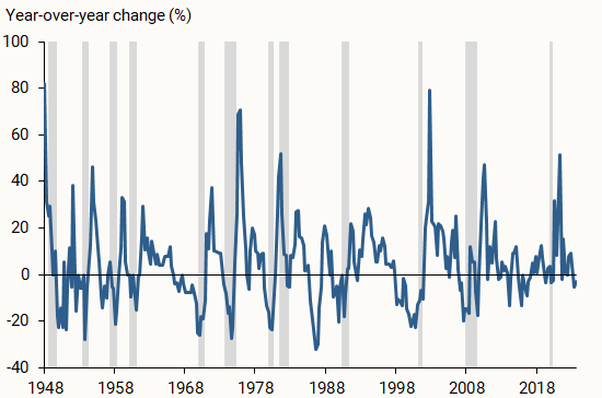
More importantly, corporate profits are an imperfect measure of a firm’s pricing power because several other factors can drive changes in profitability. For instance, much of the recent rise in corporate profits can be attributed to lower business taxes and higher subsidies from pandemic-related government support, as well as lower net interest payments due to monetary policy accommodation (Pallazzo 2023).

Instead of relying on profits as a measure of pricing power, we construct direct measures of markups based on standard economic models. Theory suggests that companies set prices as a markup over variable production costs, and that markup can be inferred from the share of a firm’s revenue spent on a given variable production factor, such as labor or intermediate goods. Over the period of data we use, we assume that the specific proportion of a company’s production costs going toward inputs does not change. If the share of a firm’s revenue used for inputs falls, it would imply a rise in the firm’s price-cost margin or markup. In our main analysis, we use industry-level data from the Bureau of Economic Analysis (BEA) to compute markups based on the share of revenue spent on intermediate inputs. Our results are similar if we instead use the share of revenue going toward labor costs.

We compare the evolution of markups to that of prices, as measured by the PCE price index, since the recovery from the pandemic. In constructing this price index, the BEA takes into account changes in product characteristics (for instance, size) that could otherwise bias the inflation measure by comparing the prices of inherently different products over time. Similarly, based upon standard economic theory, our markup measure implicitly captures changes in those characteristics (see, for example, Aghion et al. 2023).

The post-pandemic evolution of markups

We examine the evolution of markups in each industry since the third quarter of 2020, the start of the post-pandemic recovery. Figure 2 shows that some sectors, such as the motor vehicles and petroleum industries, experienced large cumulative increases in markups during the recovery. Markups also rose substantially in general merchandise, such as department stores, and for other services, such as repair and maintenance, personal care, and laundry services. Since the start of the expansion, markups in those industries rose by over 10%—comparable in size to the cumulative increases over the same period in the core PCE price index, which excludes volatile food and energy components. However, the surge in inflation through June 2022 was broad based, with prices also rising substantially outside of these sectors. Thus, understanding the importance of markups for driving inflation requires a macroeconomic perspective that examines the evolution of aggregate markups across all sectors of the economy.

Figure 2 Cumulative changes in markups for salient industries

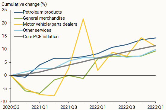
The role of aggregate markups in the economy

To assess how much markup changes contribute to movements in inflation more broadly, we use our industry-level measurements to calculate an aggregate markup at the macroeconomic level. We aggregate the cumulative changes in industry markups, applying two different weighting methods, as displayed in Figure 3. In the first method (green line), we match our industry categories to the spending categories in the core PCE price index for ease of comparison; we then use the PCE weights for each category to compute the aggregate markup. Alternatively, we use each industry’s cost weights to compute the aggregate markup (blue line). Regardless of the weighting method, Figure 3 shows that aggregate markups have stayed essentially flat since the start of the recovery, while the core PCE price index (gray line) rose by more than 10%. Thus, changes in markups are not likely to be the main driver of inflation during the recovery, which aligns with results from Glover, Mustre-del-Río, and von Ende-Becker (2023) and Hornstein (2023) using different methodologies or data. Markups also have not played much of a role in the slowing of inflation since the summer of 2022.

Figure 3 Cumulative changes in aggregate markups and prices

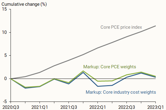
Moreover, the path of aggregate markups over the past three years is not unusual compared with previous recoveries. Figure 4 shows the cumulative changes in aggregate markups since the start of the current recovery (dark blue line), alongside aggregate markups following the 1991 (green line), 2001 (yellow line), and 2008 (light blue line) recessions. Aggregate markups have stayed roughly constant throughout all four recoveries.

Figure 4 Cumulative changes of aggregate markups in recoveries

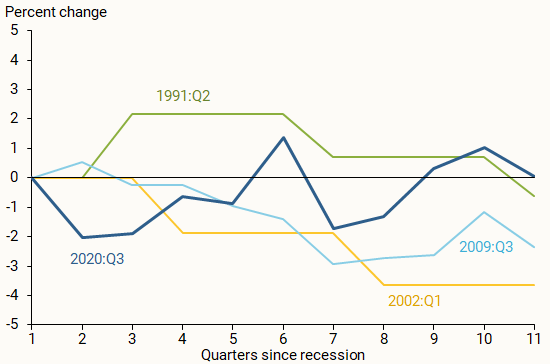
Firms’ pricing power may change over time, resulting in markup fluctuations. In this Letter , we examine whether increases in markups played an important role during the inflation surge between early 2021 and mid-2022 and if declines in markups have contributed to disinflation since then. Using industry-level data, we show that markups did rise substantially in a few important sectors, such as motor vehicles and petroleum products. However, aggregate markups—the more relevant measure for overall inflation—have stayed essentially flat since the start of the recovery. As such, rising markups have not been a main driver of the recent surge and subsequent decline in inflation during the current recovery.

Aghion, Philippe, Antonin Bergeaud, Timo Boppart, Peter J. Klenow, and Huiyu Li. 2023. “A Theory of Falling Growth and Rising Rents.”  Review of Economic Studies  90(6), pp.2,675-2,702.

Glover, Andrew, José Mustre-del-Río, and Alice von Ende-Becker. 2023. “ How Much Have Record Corporate Profits Contributed to Recent Inflation? ” FRB Kansas City Economic Review 108(1).

Hornstein, Andreas. 2023. “ Profits and Inflation in the Time of Covid .” FRB Richmond Economic Brief 23-38 (November).

Liu, Zheng, and Thuy Lan Nguyen. 2023. “ Global Supply Chain Pressures and U.S. Inflation .” FRBSF Economic Letter 2023-14 (June 20).

Palazzo, Berardino. 2023. “ Corporate Profits in the Aftermath of COVID-19 .” FEDS Notes , Federal Reserve Board of Governors, September 8.

Weber, Isabella M. and Evan Wasner. 2023. “Sellers’ Inflation, Profits and Conflict: Why Can Large Firms Hike Prices in an Emergency?” Review of Keynesian Economics 11(2), pp. 183-213.

Opinions expressed in FRBSF Economic Letter do not necessarily reflect the views of the management of the Federal Reserve Bank of San Francisco or of the Board of Governors of the Federal Reserve System. This publication is edited by Anita Todd and Karen Barnes. Permission to reprint portions of articles or whole articles must be obtained in writing. Please send editorial comments and requests for reprint permission to [email protected]

Female labor force participation

Across the globe, women face inferior income opportunities compared with men. Women are less likely to work for income or actively seek work. The global labor force participation rate for women is just over 50% compared to 80% for men. Women are less likely to work in formal employment and have fewer opportunities for business expansion or career progression. When women do work, they earn less. Emerging evidence from recent household survey data suggests that these gender gaps are heightened due to the COVID-19 pandemic.

Women’s work and GDP

Women’s work is posited to be related to development through the process of economic transformation.

Levels of female labor force participation are high for the poorest economies generally, where agriculture is the dominant sector and women often participate in small-holder agricultural work. Women’s participation in the workforce is lower in middle-income economies which have much smaller shares of agricultural activities. Finally, among high-income economies, female labor force participation is again higher, accompanied by a shift towards a service sector-based economy and higher education levels among women.

This describes the posited  U-shaped relationship  between development (proxied by GDP per capita) and female labor force participation where women’s work participation is high for the poorest economies, lower for middle income economies, and then rises again among high income economies.

This theory of the U-shape is observed globally across economies of different income levels. But this global picture may be misleading. As more recent studies have found, this pattern does not hold within regions or when looking within a specific economy over time as their income levels rise.

In no region do we observe a U-shape pattern in female participation and GDP per capita over the past three decades.

Structural transformation, declining fertility, and increasing female education in many parts of the world have not resulted in significant increases in women’s participation as was theorized. Rather, rigid historic, economic, and social structures and norms factor into stagnant female labor force participation.

Historical view of women’s participation and GDP

Taking a historical view of female participation and GDP, we ask another question: Do lower income economies today have levels of participation that mirror levels that high-income economies had decades earlier?

The answer is no.

This suggests that the relationship of female labor force participation to GDP for lower-income economies today is different than was the case decades past. This could be driven by numerous factors -- changing social norms, demographics, technology, urbanization, to name a few possible drivers.

Gendered patterns in type of employment

Gender equality is not just about equal access to jobs but also equal access for men and women to good jobs. The type of work that women do can be very different from the type of work that men do. Here we divide work into two broad categories: vulnerable work and wage work.

The Gender gap in vulnerable and wage work by GDP per capita

Vulnerable employment is closely related to GDP per capita. Economies with high rates of vulnerable employment are low-income contexts with a large agricultural sector. In these economies, women tend to make up the higher share of the vulnerably employed. As economy income levels rise, the gender gap also flips, with men being more likely to be in vulnerable work when they have a job than women.

From COVID-19 crisis to recovery

The COVID-19 crisis has exacerbated these gender gaps in employment. Although comprehensive official statistics from labor force surveys are not yet available for all economies,  emerging studies  have consistently documented that working women are taking a harder hit from the crisis. Different patterns by sector and vulnerable work do not explain this. That is, this result is not driven by the sectors in which women work or their higher rates of vulnerable work—within specific work categories, women fared worse than men in terms of COVID-19 impacts on jobs.

Among other explanations is that women have borne the brunt of the increase in the demand for care work (especially for children). A strong and inclusive recovery will require efforts which address this and other underlying drivers of gender gaps in employment opportunities.

• Research and Publications
• Projects and Operations
• Privacy Notice
• Site Accessibility
• Access to Information
• REPORT FRAUD OR CORRUPTION

Cities as Engines of Opportunities: Evidence from Brazil

Are developing-world cities engines of opportunities for low-wage earners? In this study, we track a cohort of young low-income workers in Brazil for thirteen years to explore the contribution of factors such as industrial structure and skill segregation on upward income mobility. We find that cities in the south of Brazil are more effective engines of upward mobility than cities in the north and that these differences appear to be primarily related to the exposure of unskilled workers to skilled co-workers, which in turn reflects industry composition and complexity. Our results suggest that the positive effects of urbanization depend on the skilled and unskilled working together, a form of integration that is more prevalent in the cities of southern Brazil than in northern cities. This segregation, which can decline with specialization and the division of labor, may hinder the ability of Brazil's northern cities to offer more opportunities for escaping poverty.

We acknowledge the support of Cristian Jara-Figueroa in the initial conceptualization of the empirical strategy. Barza and Viarengo gratefully acknowledges the financial support received from the Swiss National Science Foundation (Principal Investigator: Prof. Dr. Martina Viarengo; Research Grant n. 100018-176454). Hidalgo acknowledges the support of the Agence Nationale de la Recherche grant number ANR-19-P3IA-0004, the 101086712-LearnData-HORIZON-WIDERA-2022-TALENTS-01 financed by European Research Executive Agency (REA) (https://cordis.europa.eu/project/id/101086712), IAST funding from the French National Research Agency (ANR) under grant ANR-17-EURE-0010 (Investissements d'Avenir program), and the European Lighthouse of AI for Sustainability [grant number 101120237-HOR-IZON-CL4-2022-HUMAN-02]. The usual caveats apply. The views expressed herein are those of the authors and do not necessarily reflect the views of the National Bureau of Economic Research.

I have received speaking fees from organizations that organize members that invest in real estate markets, including the National Association of Real Estate Investment Managers, the Pension Real Estate Association and the Association for International Real Estate Investors.

MARC RIS BibTeΧ

Download Citation Data

Working Groups

Mentioned in the news, more from nber.

In addition to working papers , the NBER disseminates affiliates’ latest findings through a range of free periodicals — the NBER Reporter , the NBER Digest , the Bulletin on Retirement and Disability , the Bulletin on Health , and the Bulletin on Entrepreneurship  — as well as online conference reports , video lectures , and interviews .